\(\displaystyle \left[\begin{matrix}1 & 0 & -1 & 0 & 1\\0 & 1 & 1 & 0 & -1\\0 & 0 & 0 & 1 & 1\\0 & 0 & 0 & 0 & 0\end{matrix}\right]\)
Practice Final Exam Questions Solutions
1
The augmented matrix \([A \mid \mathbf{b}]\) for a linear system has been reduced to
\[ \left[\begin{array}{cccc|c} 1 & 0 & 2 & 0 & 3 \\ 0 & 1 & -1 & 0 & 1 \\ 0 & 0 & 0 & 1 & -2 \end{array}\right]. \]
Find a basis for the null space of \(A\).
Write the general solution of \(A\mathbf{x} = \mathbf{b}\) in the form particular solution plus null space.
What is the rank of \(A\)? Is \(\mathbf{b}\) in the column space of \(A\)? Briefly justify.
Solve \(A\mathbf{x} = \mathbf{0}\). From the RREF of \(A\), we have \(x_1 + 2x_3 = 0\), \(x_2 - x_3 = 0\), and \(x_4 = 0\). So column 3 is free: set \(x_3 = t\). Then \(x_1 = -2t\), \(x_2 = t\), \(x_4 = 0\). Thus \(\mathcal{N}(A) = \operatorname{span}\{ [-2, 1, 1, 0]^T \}\), and a basis is \(\{ [-2, 1, 1, 0]^T \}\).
The general solution is a particular solution plus any vector in \(\mathcal{N}(A)\). To find a particular solution, set the free variable \(x_3 = 0\). From the RREF of \([A \mid \mathbf{b}]\), we get \(x_1 = 3\), \(x_2 = 1\), \(x_4 = -2\). So a particular solution is \(\mathbf{x}_p = [3, 1, 0, -2]^T\). The general solution is \(\mathbf{x} = \mathbf{x}_p + t\,\mathbf{n}\) with \(\mathbf{n} \in \mathcal{N}(A)\), i.e. \(\mathbf{x} = [3, 1, 0, -2]^T + t[-2, 1, 1, 0]^T\), \(t \in \mathbb{R}\).
The rank of \(A\) is the number of pivot columns in the RREF of \(A\). The given RREF has pivots in columns 1, 2, and 4, so rank \(= 3\). Yes, \(\mathbf{b} \in \mathcal{C}(A)\): the system \(A\mathbf{x} = \mathbf{b}\) is consistent (we have a particular solution), so \(\mathbf{b}\) is in the column space of \(A\).
2
A directed graph has vertices \(A\), \(B\), \(C\), \(D\) and edges: \(A \to B\), \(A \to C\), \(B \to C\), \(B \to D\), \(C \to D\). (So there are 5 edges.)
Write the adjacency matrix \(A\) and the incidence matrix \(B\) (orientation: tail \(= +1\), head \(= -1\)). Use vertex order \(A, B, C, D\) and number the edges in the order listed above.
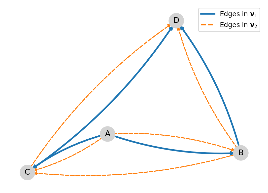
A loop in the graph is a subset of edges that form a closed path (each vertex has the same number of edges in as out along the loop). Find a basis for the set of loops by finding a basis for the null space of \(B\), and draw the graph with the basis of loops indicated. (It’s fine if the loops are not directed loops, just closed paths.)
For your reference, here is the RREF of \(B\):
- This graph does not contain any directed loops – that is, it is impossible to start at a vertex and follow a sequence of directed edges to return to the same vertex. Show that this property follows from the fact that \(A^4=\begin{bmatrix} 0 & 0 & 0 & 0 \\ 0 & 0 & 0 & 0 \\ 0 & 0 & 0 & 0 \\ 0 & 0 & 0 & 0 \end{bmatrix}\).
- Order vertices A, B, C, D. Edges: 1=A→B, 2=A→C, 3=B→C, 4=B→D, 5=C→D.
\(A = \begin{bmatrix} 0 & 1 & 1 & 0 \\ 0 & 0 & 1 & 1 \\ 0 & 0 & 0 & 1 \\ 0 & 0 & 0 & 0 \end{bmatrix}\) (rows/cols = A,B,C,D).
\(B = \begin{bmatrix} 1 & 1 & 0 & 0 & 0 \\ -1 & 0 & 1 & 1 & 0 \\ 0 & -1 & -1 & 0 & 1 \\ 0 & 0 & 0 & -1 & -1 \end{bmatrix}\) (rows = vertices A,B,C,D; columns = edges 1..5).
- \(B\) is \(4 \times 5\) and its rows sum to zero, so \(\operatorname{rank}(B)\le 3\); in fact \(\operatorname{rank}(B)=3\), hence \(\dim\mathcal{N}(B)=5-3=2\). Solving \(B\mathbf{x}=\mathbf{0}\) gives, for example, the basis \(\mathbf{v}_1=\begin{bmatrix}1\\-1\\1\\0\\0\end{bmatrix}\) and \(\mathbf{v}_2=\begin{bmatrix}0\\0\\1\\-1\\1\end{bmatrix}\). So a basis for the loop space is \(\{\mathbf{v}_1,\mathbf{v}_2\}\).
These correspond to the two closed paths \(A-B-C-A\) and \(B-C-D-B\). The signs indicate whether an edge is traversed with or against the chosen orientation of that edge.
- The \((i,j)\) entry of \(A^k\) is the number of paths of length \(k\) from vertex \(i\) to vertex \(j\).
If there are any directed cycles in the graph, then we can create a path that goes around the cycle multiple times, continuing indefinitely. Starting from a vertex on the cycle, there exists walks of every length, so at least some element of \(A^k\) must be nonzero for all \(k\).
Therefore, \(A^4 = \mathbf{0}\) implies there are no directed cycles in the graph.
3
A linear system in unknowns \(x_1, x_2, x_3, x_4\) has general solution \((4 + x_2 - 3x_4,\, x_2,\, 2 - x_4,\, x_4)\) where \(x_2\) and \(x_4\) are free. Find a minimal reduced row echelon form (augmented matrix) for this system.
From the general solution: \(x_1 = 4 + x_2 - 3x_4\), \(x_3 = 2 - x_4\), so \(x_1 - x_2 + 3x_4 = 4\) and \(x_3 + x_4 = 2\). A minimal RREF is
\[ R = \left[\begin{array}{cccc|c} 1 & -1 & 0 & 3 & 4 \\ 0 & 0 & 1 & 1 & 2 \end{array}\right]. \]
4
Find a least-squares solution to
\[ \begin{bmatrix} 1 & 0 \\ 1 & 1 \\ 1 & 2 \end{bmatrix} \begin{bmatrix} x_1 \\ x_2 \end{bmatrix} = \begin{bmatrix} 2 \\ 1 \\ 0 \end{bmatrix}. \]
Is it a genuine solution? Verify by computing the residual.
Normal equations: \(A^T A \mathbf{x} = A^T \mathbf{b}\). \(A^T A = \begin{bmatrix} 3 & 3 \\ 3 & 5 \end{bmatrix}\), \(A^T \mathbf{b} = \begin{bmatrix} 3 \\ 1 \end{bmatrix}\). Then \(\mathbf{x} = (A^T A)^{-1} A^T \mathbf{b} = [2, -1]^T\). We have \(A\mathbf{x} = [2, 1, 0]^T = \mathbf{b}\), so it is a genuine solution (residual \(\mathbf{0}\)).
5
Show that if \(A^T A \mathbf{y} = \mathbf{0}\), then \(A\mathbf{y} = \mathbf{0}\). (Hint: consider \(\|A\mathbf{y}\|^2\).)
We have \(\|A\mathbf{y}\|^2 = (A\mathbf{y})^T (A\mathbf{y}) = \mathbf{y}^T A^T A \mathbf{y}\). If \(A^T A \mathbf{y} = \mathbf{0}\), then \(\mathbf{y}^T A^T A \mathbf{y} = \mathbf{y}^T \mathbf{0} = 0\), so \(\|A\mathbf{y}\|^2 = 0\). Hence \(A\mathbf{y} = \mathbf{0}\).
6
For \(A = \begin{bmatrix} 4 & 2 \\ -1 & 1 \end{bmatrix}\), find the eigenvalues and eigenvectors, and find \(P\), \(D\) such that \(A = P D P^{-1}\).
Use (a) to write \(A^3\) in the form \(P D^3 P^{-1}\) (you may leave \(P^{-1}\) unevaluated).
What is the spectral radius of \(A\)?
Using (a), diagonalize the matrix \(A^2 - 5A + 6I\). What is the null space of \(A^2 - 5A + 6I\)? (You may use the fact that for a diagonalizable matrix, \(p(A) = P\, p(D)\, P^{-1}\) when \(p\) is a polynomial.)
Characteristic polynomial: \((\lambda-4)(\lambda-1)+2 = \lambda^2 - 5\lambda + 6 = (\lambda-2)(\lambda-3)\). So \(\lambda_1 = 2\), \(\lambda_2 = 3\). Eigenvectors: for 2, \(\mathbf{v}_1 = [1, -1]^T\); for 3, \(\mathbf{v}_2 = [2, -1]^T\). So \(P = \begin{bmatrix} 1 & 2 \\ -1 & -1 \end{bmatrix}\), \(D = \operatorname{diag}(2, 3)\).
\(A^3 = P D^3 P^{-1} = P \operatorname{diag}(8, 27) P^{-1}\).
Spectral radius \(\rho(A) = \max|\lambda| = 3\).
We have \(A = P D P^{-1}\), so \(A^2 - 5A + 6I = P(D^2 - 5D + 6I)P^{-1}\). The eigenvalues of \(A\) are 2 and 3, so \(D^2 - 5D + 6I = \operatorname{diag}(4-10+6,\, 9-15+6) = \operatorname{diag}(0,0) = 0\). Hence \(A^2 - 5A + 6I = 0\) (the zero matrix). The null space of the zero matrix is all of \(\mathbb{R}^2\).
7
A population is modeled with three life stages (e.g. juvenile, subadult, adult). The transition matrix is \[ A = \begin{bmatrix} 0 & 0 & 2 \\ 0.5 & 0 & 0 \\ 0 & 0.6 & 0 \end{bmatrix}. \]
In words, what does this model say about how individuals move between stages and reproduce in a given time step?
Starting with a population vector \(\mathbf{x}_0 = (0, 20, 50)^T\), compute the population after one and after two time steps (i.e. \(\mathbf{x}_1\) and \(\mathbf{x}_2\)).
The dominant eigenvalue of \(A\) (largest in modulus) is \(\lambda_1 \approx 0.84\). What does that tell you about the long-term behavior of the population?
Adults produce 2 juveniles per time step (and do not survive). Juveniles become subadults with probability 0.5; subadults become adults with probability 0.6. So in one step: births from adults only, then survival/transition juvenile→subadult→adult.
\(\mathbf{x}_1=A\mathbf{x}_0=(100,0,12)^T\): there are \(2\cdot 50=100\) juveniles produced by adults, \(0.5\cdot 0=0\) subadults coming from juveniles, and \(0.6\cdot 20=12\) adults coming from subadults. Then \(\mathbf{x}_2=A\mathbf{x}_1=(0,50,0)^T + (24,0,0)^T = (24,50,0)^T\).
\(|\lambda_1| < 1\) means the population decays in the long run (no stable nonzero equilibrium); the total population eventually tends to zero. (For this matrix, \(\lambda_1 = 0.6^{1/3} \approx 0.84\).)
8
Convert the difference equation \(y_{k+2} - 2y_{k+1} + y_{k} = 1\) into the form \(\mathbf{x}_{k+1} = A \mathbf{x}_k\) for some state vector \(\mathbf{x}_k\) and matrix \(A\). Because the right-hand side of the difference equation is nonzero, use a state vector that includes a constant component (e.g. a third entry equal to 1).
Solve for \(y_{k+2}\): \(y_{k+2} = 2y_{k+1} - y_{k} + 1\). Define \(\mathbf{x}_k = [y_{k}, y_{k+1}, 1]^T\). Then \(\mathbf{x}_{k+1}[1] = x_k[2]\), \(\mathbf{x}_{k+1}[2] = 2x_k[2] - x_k[1] + x_k[3]\), \(\mathbf{x}_{k+1}[3] = x_k[3]\). So \(A = \begin{bmatrix} 0 & 1 & 0 \\ -1 & 2 & 1 \\ 0 & 0 & 1 \end{bmatrix}\).
9
Suppose \(A = U \Sigma V^T\) is the SVD of a real \(m \times n\) matrix with nonzero singular values \(\sigma_1 \ge \cdots \ge \sigma_r > 0\). Let \(\mathbf{u}_i\) and \(\mathbf{v}_i\) be the \(i\)th columns of \(U\) and \(V\).
What is \(A \mathbf{v}_1\) in terms of \(\sigma_1\) and \(\mathbf{u}_1\)?
What is \(A^T A \mathbf{v}_1\)?
Give a formula for the least-squares solution(s) to \(A\mathbf{x} = \mathbf{b}\) in terms of \(U\), \(\Sigma\), \(V\), and \(\mathbf{b}\).
Suppose \(r = n\) (full column rank). Describe the solution set of \(A\mathbf{x} = \mathbf{0}\). What does that imply about the least-squares solution to \(A\mathbf{x} = \mathbf{b}\)?
\(A\mathbf{v}_1 = \sigma_1 \mathbf{u}_1\).
\(A^T A \mathbf{v}_1 = \sigma_1^2 \mathbf{v}_1\).
\(\mathbf{x} = V \Sigma^+ U^T \mathbf{b} + \mathbf{n}\) where \(\Sigma^+\) has \(1/\sigma_i\) on the diagonal for \(i=1,\ldots,r\) and \(\mathbf{n} \in \mathcal{N}(A)\) (or: \(\mathbf{x} = A^+ \mathbf{b} + \mathbf{n}\) with \(A^+ = V \Sigma^+ U^T\)).
If \(r = n\), the null space of \(A\) is \(\{\mathbf{0}\}\) (only the zero vector). So the least-squares solution is unique: \(\mathbf{x} = A^+ \mathbf{b}\).
10
Let \(A = \begin{bmatrix} 1 & 2 & 1 \\ 0 & 1 & 1 \\ 1 & 3 & 2 \end{bmatrix}\).
Find the reduced row echelon form of \(A\) and its rank.
Find a basis for the column space of \(A\).
Determine which of the following vectors is in the column space of \(A\) and, if so, express it as a linear combination of the columns of \(A\): \(\mathbf{b}_1 = [0, 0, 1]^T\), \(\mathbf{b}_2 = [1, 2, 3]^T\).
RREF: \(\begin{bmatrix} 1 & 0 & -1 \\ 0 & 1 & 1 \\ 0 & 0 & 0 \end{bmatrix}\). Rank = 2.
Pivot columns 1 and 2. Basis: \(\mathbf{a}_1 = [1, 0, 1]^T\), \(\mathbf{a}_2 = [2, 1, 3]^T\).
Solve \(A\mathbf{x} = \mathbf{b}_1\) and \(A\mathbf{x} = \mathbf{b}_2\). The system for \(\mathbf{b}_1\) has augmented matrix with last row [0 0 0 | 1], so inconsistent: \(\mathbf{b}_1 \notin \mathcal{C}(A)\). For \(\mathbf{b}_2\), one particular solution is \(x_3 = 0\), \(x_2 = 2\), \(x_1 = -3\), so \(\mathbf{b}_2 = -3\mathbf{a}_1 + 2\mathbf{a}_2 \in \mathcal{C}(A)\).
11
A bandpass filter attenuates both the lowest frequencies (near DC, \(k=0\)) and the highest frequencies (near Nyquist, \(k = N/2\) when \(N\) is even), and passes a band of frequencies in the middle. So the filter’s gain is (or is close to) zero at \(k=0\) and at \(k=N/2\), and is nonzero for some \(k\) strictly between \(0\) and \(N/2\).
A signal is sampled every \(T_s = 1/6\) s (sampling rate 6 Hz) and we take \(N = 6\) samples (1 s of data). There are \(N = 6\) frequency indices \(k = 0, 1, \ldots, 5\), with corresponding frequencies \(f_k\) (in Hz): \(0\), \(1\), \(2\), \(3\) (Nyquist), \(-2\), \(-1\).
- You would like to design a bandpass filter that passes signals with frequencies between 0.5 Hz and 2.5 Hz. Write down a simple example of the six gains \(H[0], \ldots, H[5]\) for such a filter.
(For the negative frequencies, use the same filter value H[k] as for the corresponding positive frequency.)
- Suppose your signal is \(x[n] = (1, 0, 1, 1, 1, 0)\) with DFT coefficients \(X_0, \ldots, X_5\) equal to \(4, -1, 1, 2, 1, -1\) respectively. Using the transformation from lecture (below), write down the \(n\)-th entry of the filtered signal (that is, \(y[n]\)) as a sum of terms involving complex exponentials. You don’t need to do any trigonometric simplifications. \[ \mathcal{F}_h(\mathbf{x}) = \frac{1}{N} \sum_{k=0}^{N-1} X_k H(\zeta_k) \mathbf{f}_k, \]
where \(\zeta_k = 2\pi k/N\) and \(H(\zeta_k)\) is the filter gain at frequency index \(k\) (the values \(H[0], \ldots, H[5]\) from part (a)).
- The filter can also be specified by its time-domain coefficients \(h[0], h[1], \ldots, h[N-1]\), with the usual DFT relation \(H[k] = \sum_{n=0}^{N-1} h[n] e^{-i 2\pi k n / N}\). How would you recover the coefficients \(h[n]\) from the gains \(H[k]\)? (State the formula or the name of the operation.)
We need zero gain at 0 Hz (\(k=0\)) and at 3 Hz Nyquist (\(k=3\)), so \(H[0] = 0\) and \(H[3] = 0\). The other frequency indices (\(k=1,2\) for 1 Hz and 2 Hz, and \(k=4,5\) for \(-2\) Hz and \(-1\) Hz) should be nonzero. One simple example: \(H = [0, 1, 1, 0, 1, 1]\) (zero at 0 Hz and 3 Hz, gain 1 at \(\pm 1\) Hz and \(\pm 2\) Hz).
Using \(H[0]=H[3]=0\) and \(H[1]=H[2]=H[4]=H[5]=1\) from (a), the filtered output has DFT coefficients \(Y_k = X_k H(\zeta_k)\) equal to \((0, -1, 1, 0, 1, -1)\). The \(n\)-th entry of the filtered signal is \(y[n] = \frac{1}{N}\sum_{k=0}^{N-1} Y_k \, e^{i 2\pi k n/N}\), so \[ y[n] = \frac{1}{6}\left( 0 + (-1)e^{i \pi n/3} + (1)e^{i 2\pi n/3} + 0 + (1)e^{i 4\pi n/3} + (-1)e^{i 5\pi n/3} \right). \] (No trigonometric simplification required.)
The coefficients are given by the inverse DFT of the sequence \(H[0], \ldots, H[N-1]\): \[ h[n] = \frac{1}{N} \sum_{k=0}^{N-1} H[k]\, e^{i 2\pi k n / N}, \quad n = 0, \ldots, N-1. \] So: apply the inverse DFT to the vector of gains to get the filter coefficients in time.