A simplification

Outline for today

• The Fourier Series
• Discrete Fourier Transform
• Applications of the DFT

The Fourier Series

The Fourier series

The Fourier series of a function is an expansion into sines and cosines:

f(x)=a_{0}+a_{1} \cos x+b_{1} \sin x+a_{2} \cos 2 x+b_{2} \sin 2 x+\cdots

. . .

How do we find the coefficients a_{0}, a_{1}, b_{1}, a_{2}, b_{2}, \ldots?

. . .

We use orthogonality. The functions \cos x, \cos 2 x, \cos 3 x, \ldots are orthogonal on [0,2 \pi]… Same is true for the sines.

. . .

To compute a coefficient like b_{1}, multiply both sides by the corresponding function \sin x and integrate from 0 to 2 \pi. In other words, take the inner product of both sides with \sin x :

\int_{0}^{2 \pi} f(x) \sin x d x=a_{0} \int_{0}^{2 \pi} \sin x d x+a_{1} \int_{0}^{2 \pi} \cos x \sin x d x+b_{1} \int_{0}^{2 \pi}(\sin x)^{2} d x+\cdots

b_{1}=\frac{\int_{0}^{2 \pi} f(x) \sin x d x}{\int_{0}^{2 \pi}(\sin x)^{2} d x}=\frac{(f, \sin x)}{(\sin x, \sin x)}

Analogy with projections

The component of the vector b along the line spanned by a is b^{\mathrm{T}} a / a^{\mathrm{T}} a.

A Fourier series is projecting f(x) onto \sin x. Its component p in this direction is exactly b_{1} \sin x.

Euler’s formula

The complex exponential e^{i x} is a combination of \cos x and \sin x:

e^{i x}=\cos x+i \sin x

So we can rewrite the Fourier series using complex exponentials:

f(x)=c_{0}+c_{1} e^{i x}+c_{2} e^{2 i x}+\cdots = \sum_k c_k\cdot e^{i k x}

pause

The coefficients c_{0}, c_{1}, c_{2}, \ldots are related to the a’s and b’s.

For example, c_{1}=a_{1}-i b_{1}.

The formula for finding the coefficients c_{k} is the same as before, but now we use the complex exponential functions e^{i k x} instead of the sines and cosines:

c_{k}=\int_{0}^{2 \pi} f(x) e^{-i k x} d x

Discrete Fourier Transform

Discrete Fourier Series

What if we have only a series of N discrete values y_{0}, y_{1}, y_{2}, \ldots, instead of a continuous function f(x)?

. . .

First, we imagine that the values are periodic, with period N. So it’s as if they are repeating beyond the N values we have.

. . .

Then we can identify a natural period N, and rewrite x=2 \pi n / N, so the discrete Fourier series becomes

\begin{align} y[n] = \sum_k c[k]\cdot e^{i 2\pi k \frac{n}{N}} \end{align}

. . .

In matrix form, \mathbf{y} = F \mathbf{c}

where

\begin{align} \begin{bmatrix} y_0 \\ y_1 \\ y_2 \\ \vdots \\ y_{N-1} \end{bmatrix} = F c = \begin{bmatrix} 1 & 1 & 1 & \ldots & 1 \\ 1 & e^{-i 2\pi/N} & e^{-i 4\pi/N} & \ldots & e^{-i 2\pi (N-1)/N} \\ 1 & e^{-i 4\pi/N} & e^{-i 8\pi/N} & \ldots & e^{-i 4\pi (N-1)/N} \\ \vdots & \vdots & \vdots & \ddots & \vdots \\ 1 & e^{-i 2\pi(N-1)/N} & e^{-i 4\pi(N-1)/N} & \ldots & e^{-i 2\pi(N-1)(N-1)/N} \end{bmatrix} \begin{bmatrix}c_0 \\ c_1 \\ c_2 \\ \vdots \\ c_{N-1}\end{bmatrix} \end{align}

DFT matrix

\begin{align} \begin{bmatrix} y_0 \\ y_1 \\ y_2 \\ \vdots \\ y_{N-1} \end{bmatrix} = F c = \begin{bmatrix} 1 & 1 & 1 & \ldots & 1 \\ 1 & e^{-i 2\pi/N} & e^{-i 4\pi/N} & \ldots & e^{-i 2\pi (N-1)/N} \\ 1 & e^{-i 4\pi/N} & e^{-i 8\pi/N} & \ldots & e^{-i 4\pi (N-1)/N} \\ \vdots & \vdots & \vdots & \ddots & \vdots \\ 1 & e^{-i 2\pi(N-1)/N} & e^{-i 4\pi(N-1)/N} & \ldots & e^{-i 2\pi(N-1)(N-1)/N} \end{bmatrix} \begin{bmatrix}c_0 \\ c_1 \\ c_2 \\ \vdots \\ c_{N-1}\end{bmatrix} \end{align}

Visualization

From Wikipedia, Original upload by en:User:Glogger, CC BY-SA 3.0 http://creativecommons.org/licenses/by-sa/3.0/, via Wikimedia Commons

Finding the Fourier coefficients

How can we find the Fourier coefficients? . . .

By analogy with the continuous case,

c_{k}=\int_{0}^{2 \pi} f(x) e^{-i k x} d x

We will replace the integral by a sum over the discrete values y_{0}, y_{1}, y_{2}, \ldots.

c[k]= \frac{1}{N} \sum_{n=0}^{N-1} y[n] e^{-i 2 \pi k n / N}, \quad \text{for } k=0,1,2, \ldots, N-1

This defines a matrix F^\prime given as

F^\prime = \frac{1}{N}\begin{bmatrix} 1 & 1 & 1 & \ldots & 1 \\ 1 & e^{i 2\pi/N} & e^{i 4\pi/N} & \ldots & e^{i 2\pi (N-1)/N} \\ 1 & e^{i 4\pi/N} & e^{i 8\pi/N} & \ldots & e^{i 4\pi (N-1)/N} \\ \vdots & \vdots & \vdots & \ddots & \vdots \\ 1 & e^{i 2\pi(N-1)/N} & e^{i 4\pi(N-1)/N} & \ldots & e^{i 2\pi(N-1)(N-1)/N} \end{bmatrix}

Note: this is \frac{1}{N} times the complex conjugate of the matrix F: F^\prime = \frac{1}{N} F^*.

Inverse DFT

We have just shown two things:

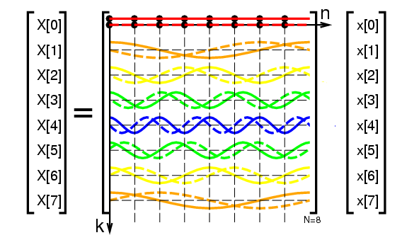
1. The DFT can be written as a matrix-vector product \mathbf{y} = F \mathbf{c}.

2. The coefficients \mathbf{c} can be found by \mathbf{c} = F^\prime \mathbf{y}.

3. But of course it is also true from 1 that if F is invertible, that \mathbf{c} = F^{-1} \mathbf{y}. Therefore, F^{-1} = F^\prime=\frac{1}{N} F^*.

4. This means that F is unitary. Its rows and columns are orthogonal.

A concrete example

Let’s take an example with N=4 and y=(2, 4, 6, 8).

. . .

We want to find coefficients c_0, c_1, c_2, c_3 such that our Fourier series correctly reproduces the input values at each of the four points.

. . .

(We can’t find more than 4 coefficients because we only have 4 points of data.)

. . .

\begin{align} y[n] = \sum_k c[k]\cdot e^{i 2\pi k \frac{n}{N}} \end{align}

. . .

\begin{aligned} c_{0}+c_{1} e^{i x}+c_{2} e^{2 i x}+c_{3} e^{3 i x}=\left\{\begin{array}{lll} 2 & \text { at } & x=0 \\ 4 & \text { at } & x=\pi / 2 \\ 6 & \text { at } & x=\pi \\ 8 & \text { at } & x=3 \pi / 2 \end{array}\right) \end{aligned}

Make a table. Note that i^2 = i^6 = -1, i^3 = i^7 = -i, and i^4 = 1.

For n = 0:

k	i 2\pi k \times 0	e^{i 2\pi k \times 0}
0	0	1
1	0	1
2	0	1
3	0	1

For n = 1:

k	i 2\pi k \frac{1}{4}	e^{i 2\pi k \frac{1}{4}}
0	0	1
1	i\pi/2	i
2	i\pi	-1=i^2
3	3i\pi/2	-i=i^3

For n = 2:

k	i 2\pi k \frac{2}{4}	e^{i 2\pi k \frac{2}{4}}
0	0	1
1	i\pi	-1=i^2
2	2i\pi	1=i^4
3	3i\pi	-1=i^6

For n = 3:

k	i 2\pi k \frac{3}{4}	e^{i 2\pi k \frac{3}{4}}
0	0	1
1	3i\pi/2	-i=i^3
2	3i\pi	-1 = i^6
3	9i\pi/2	i = i^9

Solving for the coefficients

\begin{align*} & c_{0}+c_{1}+c_{2}+c_{3}=2 \\ & c_{0}+i c_{1}+i^{2} c_{2}+i^{3} c_{3}=4 \\ & c_{0}+i^{2} c_{1}+i^{4} c_{2}+i^{6} c_{3}=6 \\ & c_{0}+i^{3} c_{1}+i^{6} c_{2}+i^{9} c_{3}=8 \end{align*}

In other words, F c = y for

F=\left[\begin{array}{cccc} 1 & 1 & 1 & 1 \\ 1 & i & i^{2} & i^{3} \\ 1 & i^{2} & i^{4} & i^{6} \\ 1 & i^{3} & i^{6} & i^{9} \end{array}\right]

Check that F F^\prime = I:

\begin{aligned} F F^\prime =\frac{1}{4}\left[\begin{array}{cccc} 1 & 1 & 1 & 1 \\ 1 & i & i^{2} & i^{3} \\ 1 & i^{2} & i^{4} & i^{6} \\ 1 & i^{3} & i^{6} & i^{9} \end{array}\right]\left[\begin{array}{cccc} 1 & 1 & 1 & 1 \\ 1 & (-i) & (-i)^{2} & (-i)^{3} \\ 1 & (-i)^{2} & (-i)^{4} & (-i)^{6} \\ 1 & (-i)^{3} & (-i)^{6} & (-i)^{9} \end{array}\right]=I \end{aligned}

Check in Sympy:

F:

\displaystyle \left[\begin{matrix}1 & 1 & 1 & 1\\1 & i & -1 & - i\\1 & -1 & 1 & -1\\1 & - i & -1 & i\end{matrix}\right]

F prime:

\displaystyle \left[\begin{matrix}0.25 & 0.25 & 0.25 & 0.25\\0.25 & - 0.25 i & -0.25 & 0.25 i\\0.25 & -0.25 & 0.25 & -0.25\\0.25 & 0.25 i & -0.25 & - 0.25 i\end{matrix}\right]

F F prime:

\displaystyle \left[\begin{matrix}1.0 & 0 & 0 & 0\\0 & 1.0 & 0 & 0\\0 & 0 & 1.0 & 0\\0 & 0 & 0 & 1.0\end{matrix}\right]

Notice that our matrix F had many terms which were exponents of i.

In general, we can simplify the matrix F by defining w = e^{i 2\pi/N}. This is the Nth “primitive root of unity”, so that w^N = 1.

. . .

For N = 4, w = e^{i \pi/2} = i.

. . .

Write the first few terms of this: \left[\begin{array}{ccccc} 1 & 1 & 1 & \cdot & 1 \\ 1 & w & w^{2} & \cdot & w^{n-1} \\ 1 & w^{2} & w^{4} & \cdot & w^{2(n-1)} \\ \cdot & \cdot & \cdot & \cdot & \cdot \\ 1 & w^{n-1} & w^{2(n-1)} & \cdot & w^{(n-1)^{2}} \end{array}\right]\left[\begin{array}{c} c_{0} \\ c_{1} \\ c_{2} \\ \cdot \\ c_{n-1} \end{array}\right]=\left[\begin{array}{c} y_{0} \\ y_{1} \\ y_{2} \\ \cdot \\ y_{n-1} \end{array}\right], \quad w = e^{i 2\pi/n}

Simplest form of Fourier matrix

Then we can write the Fourier equation as

\left[\begin{array}{ccccc} 1 & 1 & 1 & \cdot & 1 \\ 1 & w & w^{2} & \cdot & w^{n-1} \\ 1 & w^{2} & w^{4} & \cdot & w^{2(n-1)} \\ \cdot & \cdot & \cdot & \cdot & \cdot \\ 1 & w^{n-1} & w^{2(n-1)} & \cdot & w^{(n-1)^{2}} \end{array}\right]\left[\begin{array}{c} c_{0} \\ c_{1} \\ c_{2} \\ \cdot \\ c_{n-1} \end{array}\right]=\left[\begin{array}{c} y_{0} \\ y_{1} \\ y_{2} \\ \cdot \\ y_{n-1} \end{array}\right], \quad w = e^{i 2\pi/n}

Terminology

We call the matrix F the DFT (Discrete Fourier Transform) matrix. It is a square unitary matrix of size N \times N.

The matrix F^\prime is the inverse DFT matrix. It is the complex conjugate of F divided by N.

Summary

1. The DFT can be written as a matrix-vector product \mathbf{y} = F \mathbf{c}.

2. The coefficients \mathbf{c} can be found by \mathbf{c} = F^\prime \mathbf{y}.

3. F is easy to compute, with a simple formula for each entry.

4. (There’s actually a really really fast way to compute the DFT using the FFT algorithm.)

Applications of the DFT

Filtering

The DFT is used in many applications, but one of the most common is filtering.

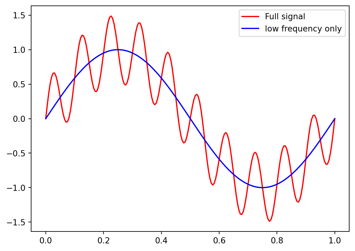
For example, suppose we have a signal that is a sum of two sinusoids:

f(x) = \sin(2\pi x) + 0.5 \sin(20\pi x)

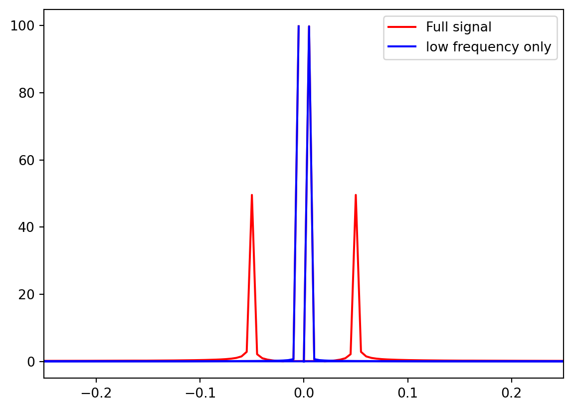
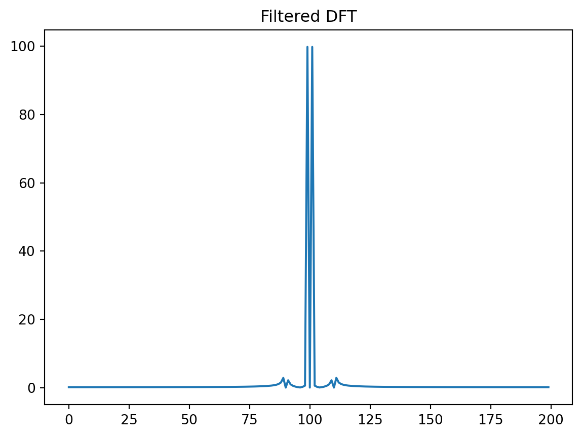
What’s the DFT of this signal?

from scipy.fft import fft, fftshift
yf = fft(y)
yfalone = fft(yalone)
# make a non connected plot of yf

plt.plot(np.fft.fftfreq(200),np.abs(yf), color='red')
plt.plot(np.fft.fftfreq(200),np.abs(yfalone), color='blue')
plt.xlim(-0.25, 0.25)
plt.legend(['Full signal', 'low frequency only'])
plt.show()

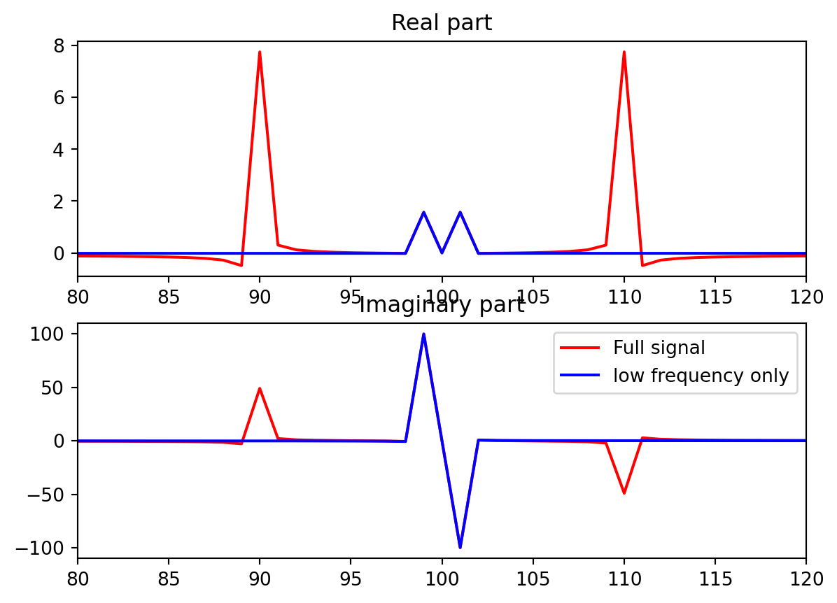
What’s with the double peaks?

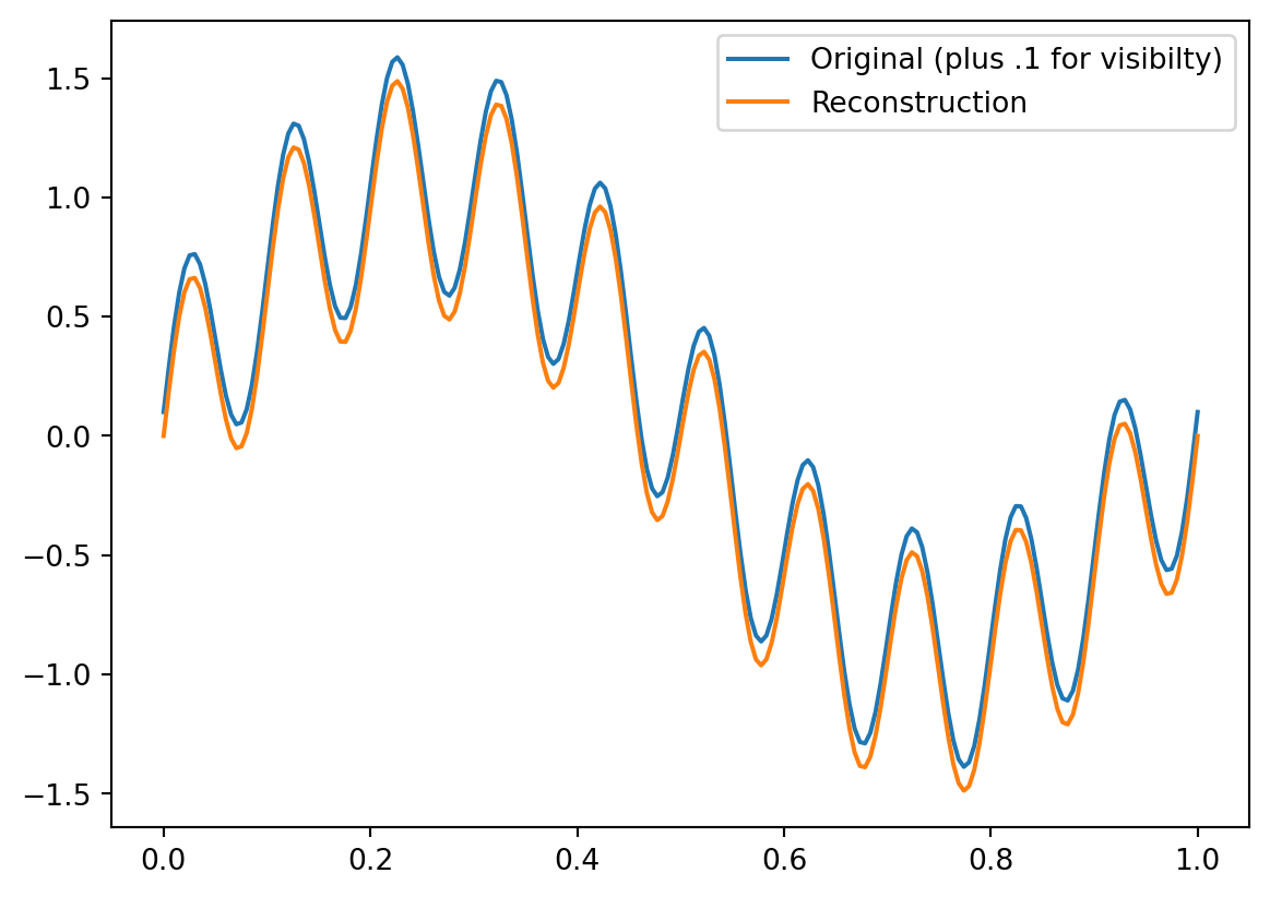
Reconstruct the signal

We can reconstruct the signal by taking the inverse DFT.

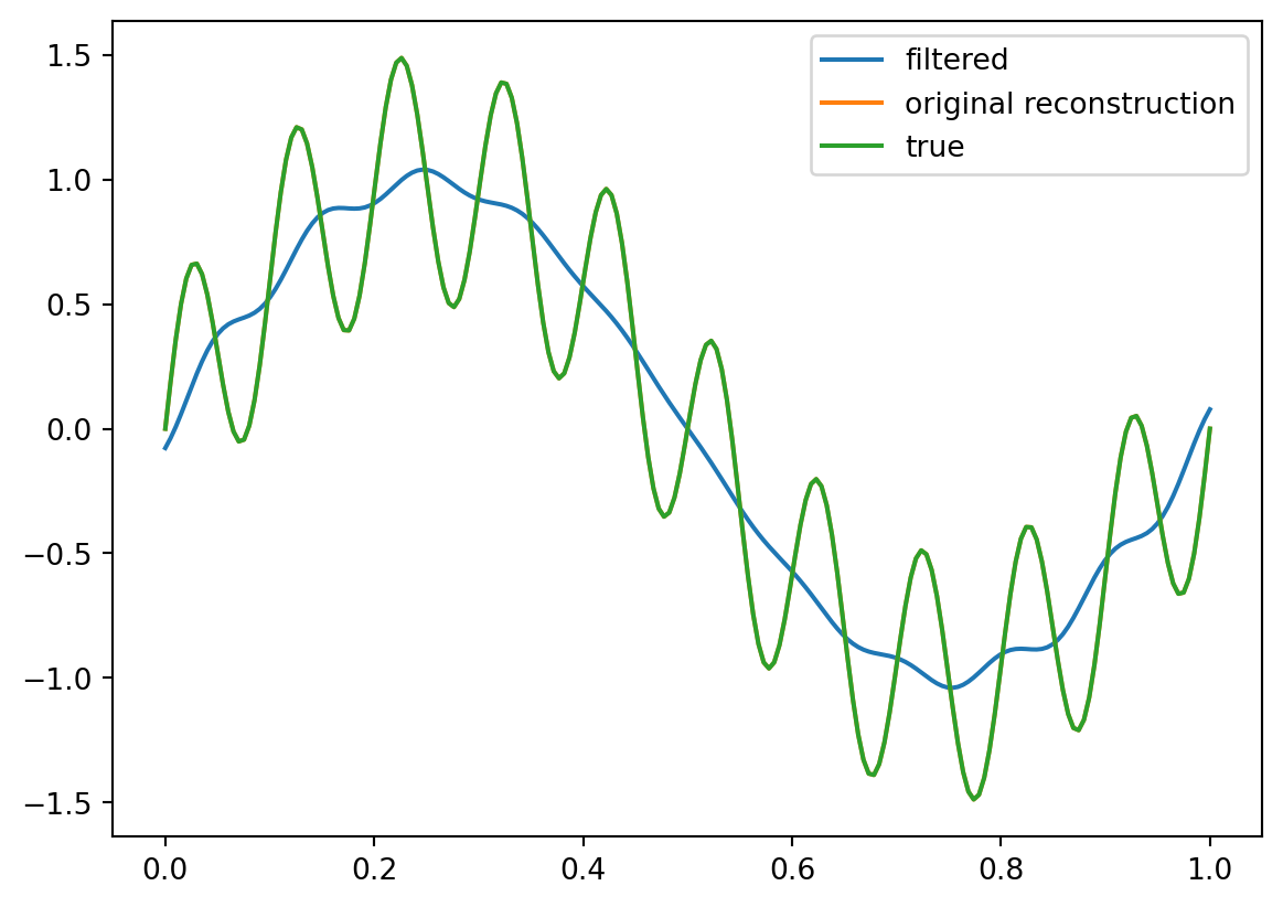
Low-pass filtering

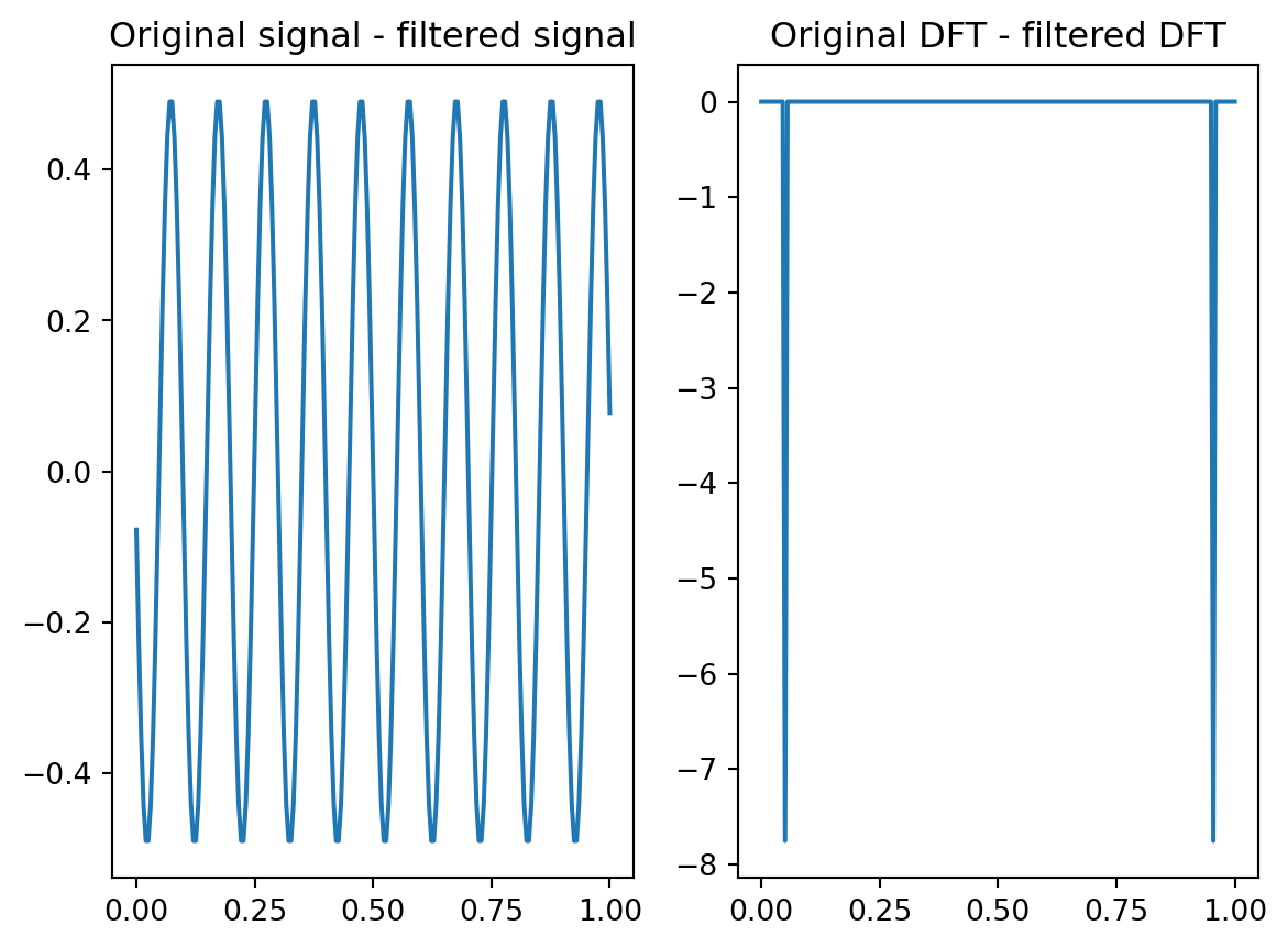
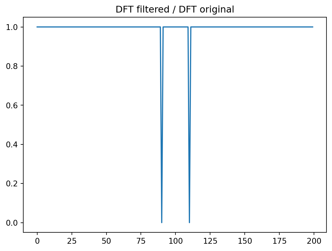
What if we just zero out the coefficient corresponding to the second sinusoid:

yf_new = yf.copy()
yf_new[190] = 0
yf_new[10] = 0
plt.plot(np.abs(fftshift(yf_new)))
plt.title('Filtered DFT')
plt.show()

Compute the inverse DFT:

It’s pretty good!

Try one more thing. Can we describe the change in the DFT as a multiplicative vector? We sure can.

So we can describe the new DVD as the old DFT multiplied by a vector of 1s and 0s.

The total process went like this:

1. Take the DFT of the signal.
2. Multiply the DFT by a vector of 1s and 0s to filter out the high frequency.
3. Take the inverse DFT to get the filtered signal.

Filtering as convolution

Suppose we have a signal and we’d like to try to filter out the high frequencies, but we don’t know which ones they are.

We could try with a simple filter like [1, 1, 1, 1, 1]/5. This is a simple moving average filter.

That means that we replace each point in the signal with the average of the 5 points before it.

Mathematically, this is:

f_{\text{filtered}}[n] = \sum_{m=0}^{4} f[n-m]/5

OK. We note that this can also be written as a convolution, between the signal and the vector h = [1, 1, 1, 1, 1, 0, 0, 0, ...]/5., where we have padded the vector with zeros so that it is the same length as the signal vector.

That is, h_0 = 1/5, h_1 = 1/5, h_2 = 1/5, h_3 = 1/5, h_4 = 1/5, and h_5 = 0, all the way to h_n=0.

Then we can write this as:

f_{\text{filtered}}[n] = \sum_{m=0}^{n} f[n-m] h[m]

This operation is called convolution.

It’s messy to compute the convolution directly. But we can do it in the Fourier domain…

The convolution theorem

The convolution of two signals f and h is the inverse DFT of the product of the DFTs of f and h.

In other words, if f = \text{ifft}(F) and h = \text{ifft}(H), then the convolution of f and h is \text{ifft}(F \cdot H).

That’s much easier to calculate – only a dot product!

Proof

(fill in if I have time)

Example

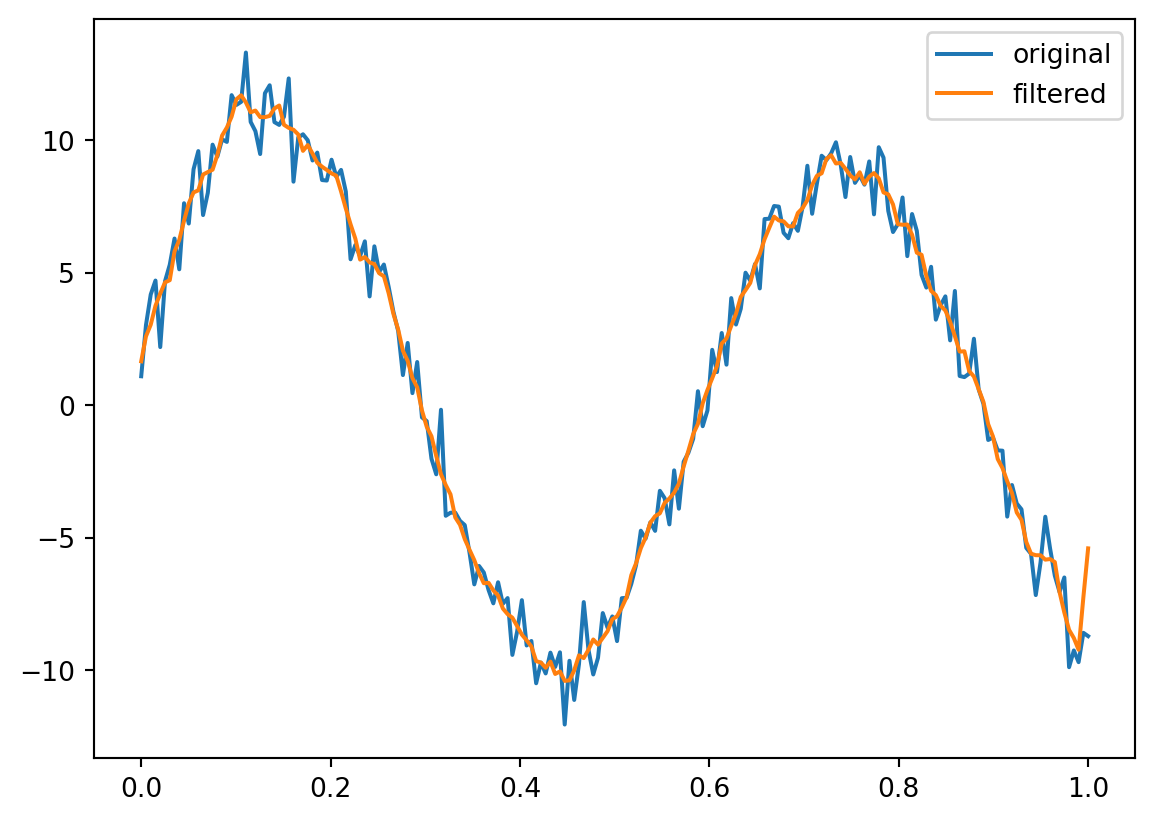
Let’s take the signal from before, f(x) = \sin(2\pi x) + 0.5 \sin(20\pi x), and filter it with the moving average filter h = [1, 1, 1, 1, 1]/5.

from scipy.signal import convolve
N = 200
x = np.linspace(0, 1, N)
y = np.sin(2*np.pi*x) + 10*np.sin(3.3*np.pi*x+.2)+ 10*np.random.normal(0, 0.1, N)
h = np.array([1, 1,1,1,1])/5
y_filtered = convolve(y, h, mode='same')
plt.plot(x, y, label='original')
plt.plot(x, y_filtered, label='filtered')
plt.legend()
plt.show()

Now try it again using the convolution theorem.

Steps:

1. Take the DFT of the signal.
2. Pad the filter with zeros to make it the same length as the signal.
3. Take the DFT of the filter.
4. Multiply the two DFTs.
5. Take the inverse DFT to get the filtered signal.
6. Done!

yf = fft(y)
hf = fft(h, N) # pad h with zeros
y_filtered = ifft(yf*hf)
plt.plot(x, y, label='original')
plt.plot(x, y_filtered, label='filtered')
plt.legend()
plt.show()

Then we can take the inverse DFT to get the filtered signal.