Ch5 Lecture 4

SVD on matrices of data

Example: Height and weight

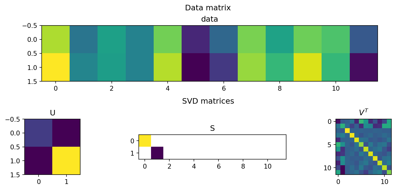
\(A^T=\left[\begin{array}{rrrrrrrrrrrr}2.9 & -1.5 & 0.1 & -1.0 & 2.1 & -4.0 & -2.0 & 2.2 & 0.2 & 2.0 & 1.5 & -2.5 \\ 4.0 & -0.9 & 0.0 & -1.0 & 3.0 & -5.0 & -3.5 & 2.6 & 1.0 & 3.5 & 1.0 & -4.7\end{array}\right]\)

Plotting

<Figure size 960x480 with 0 Axes>

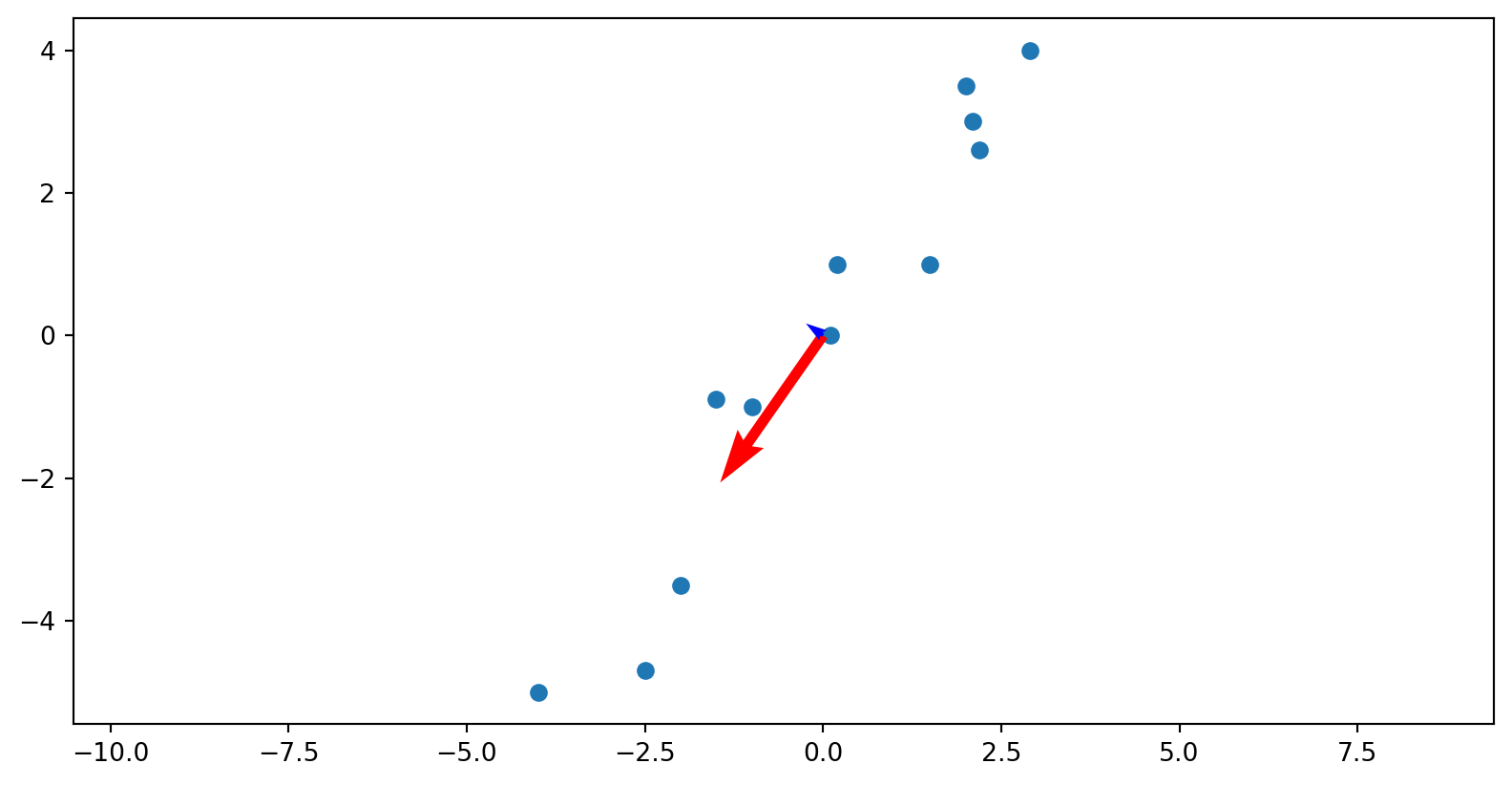
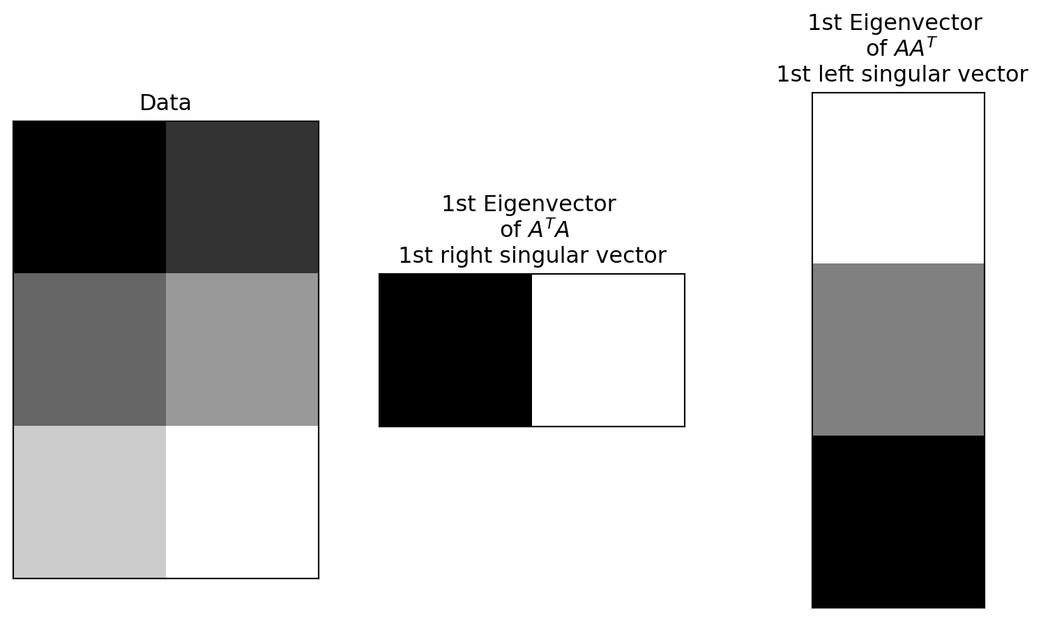
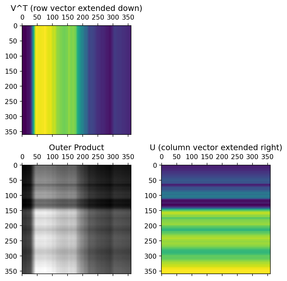
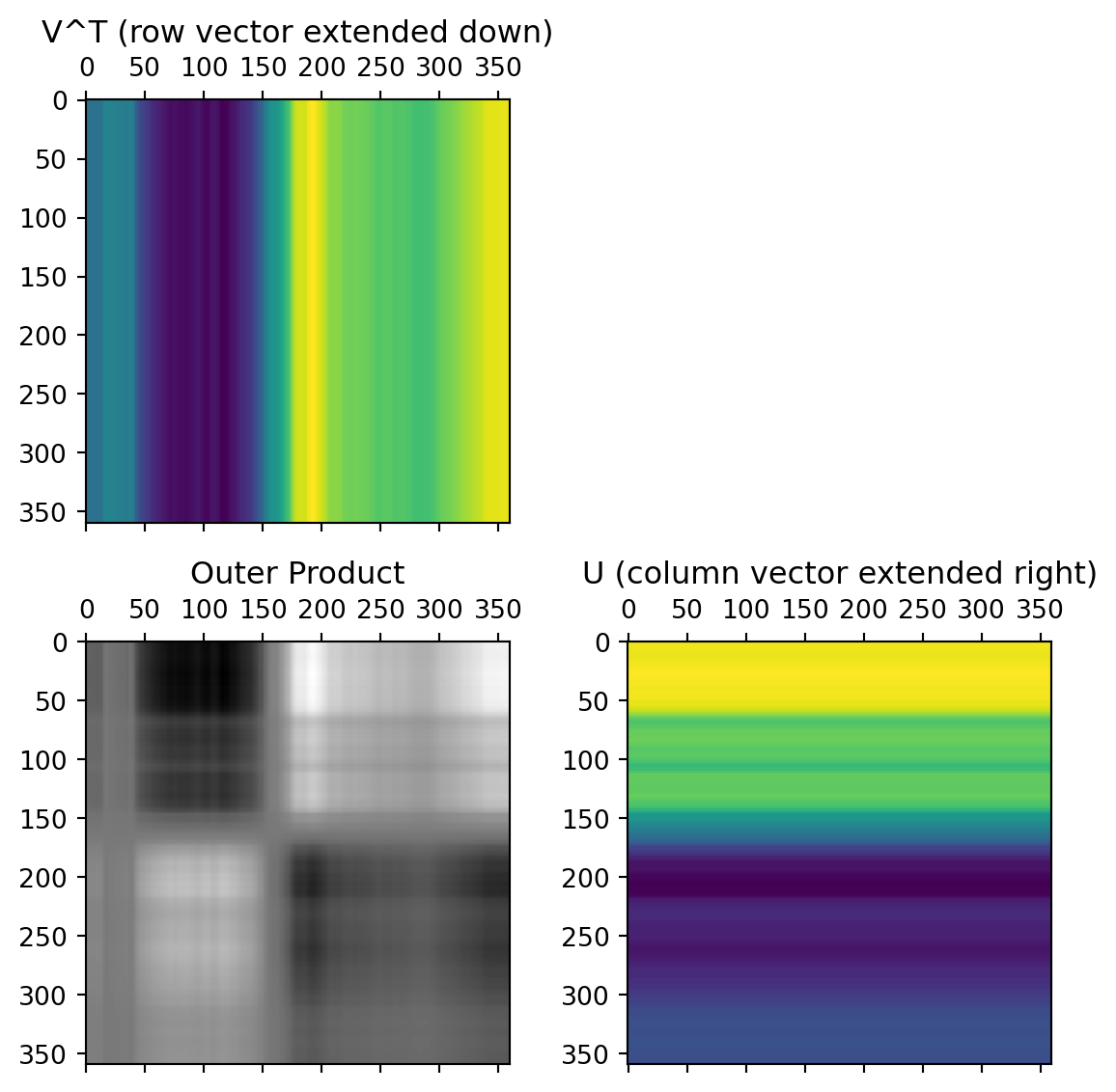
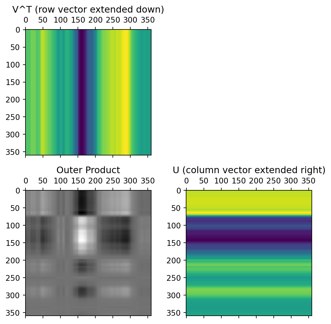
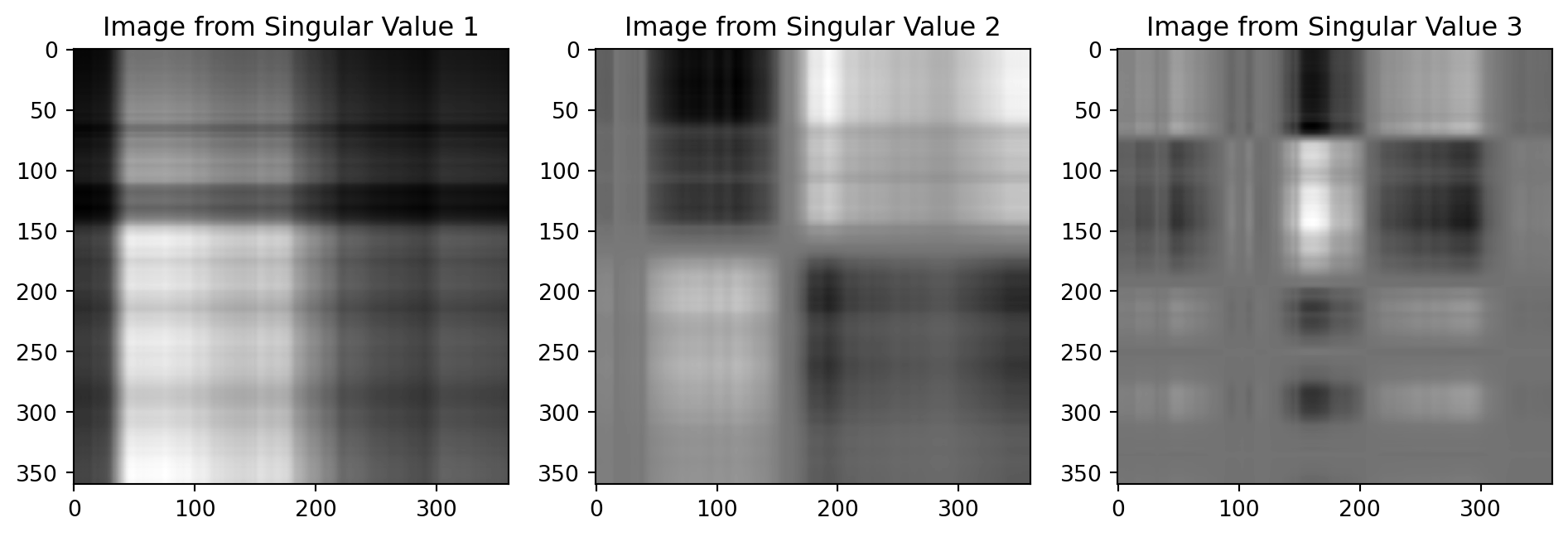
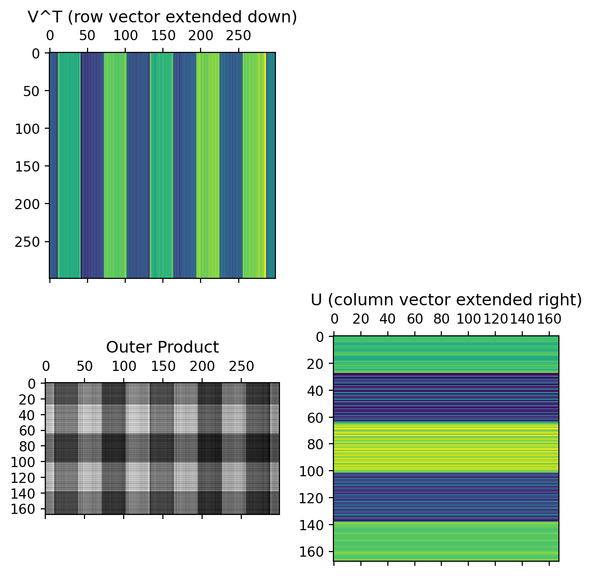
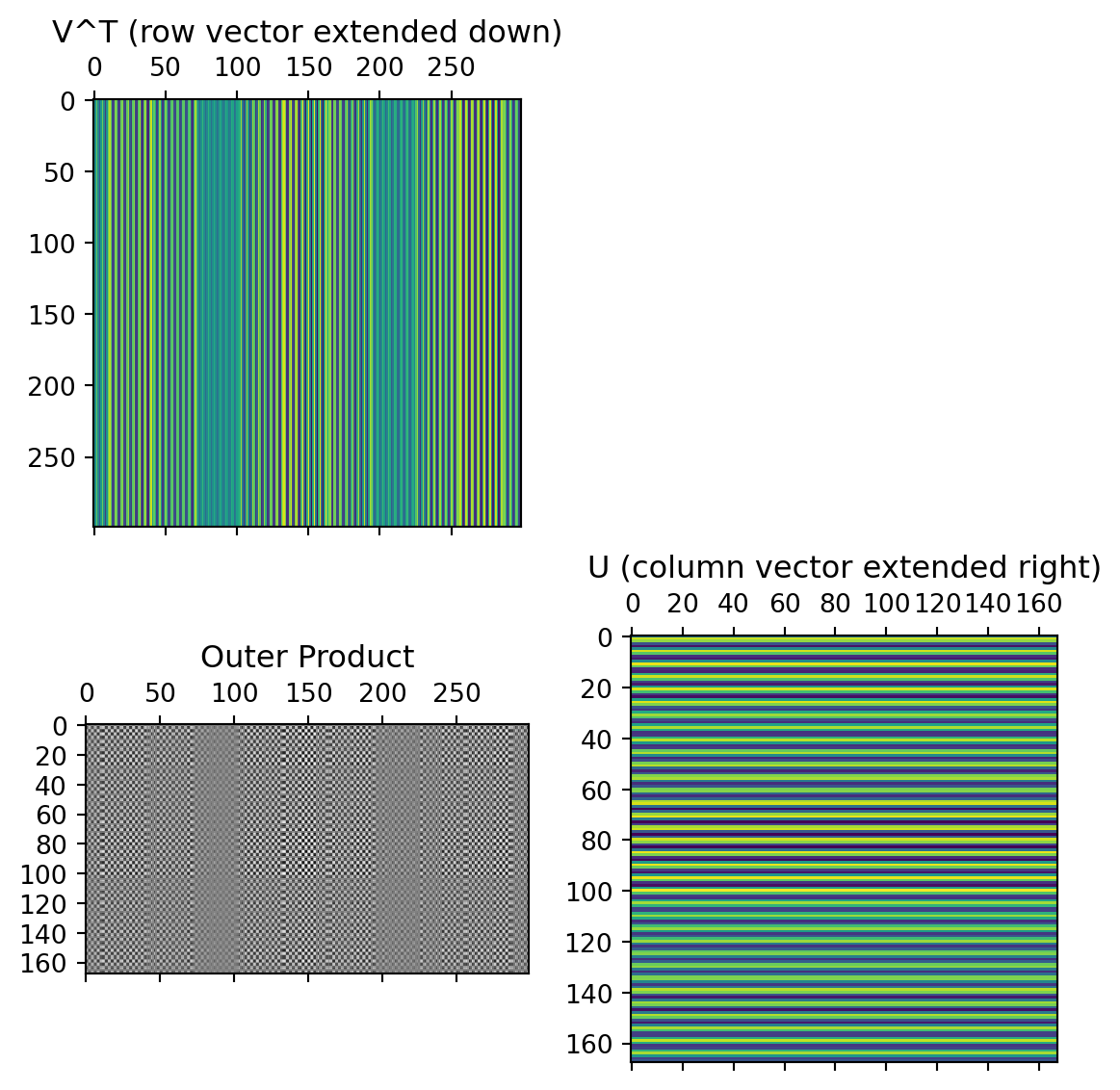
The columns of the U matrix, graphically:

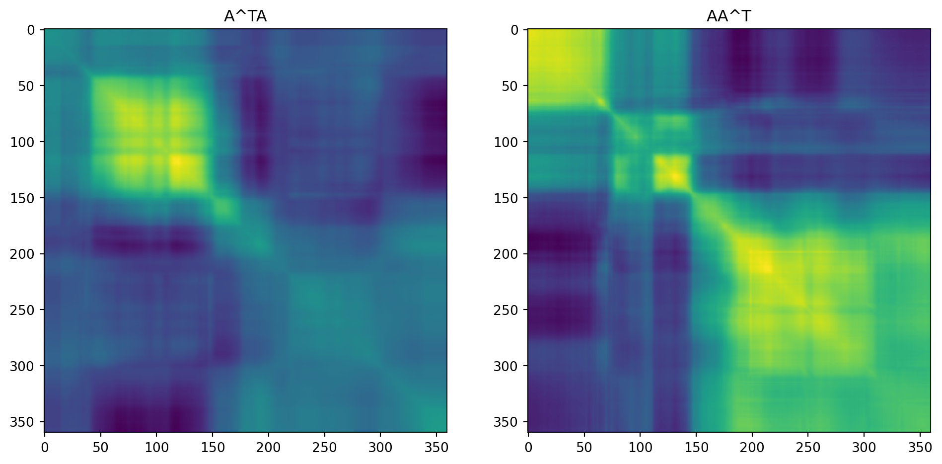
U captures relationships between the rows of the data matrix.

Since there are only two rows, only 2x2 matrix needed to capture all the relationships.

The first two rows of the \(V^T\) matrix

V captures relationships between the columns of the data matrix. 12x12 possible values, but only 12x2 needed to capture all the relationships.

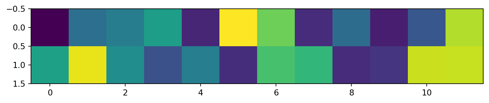
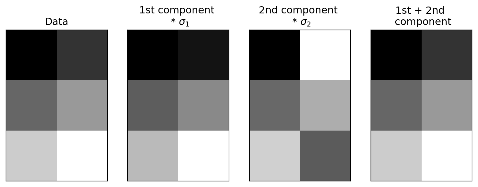
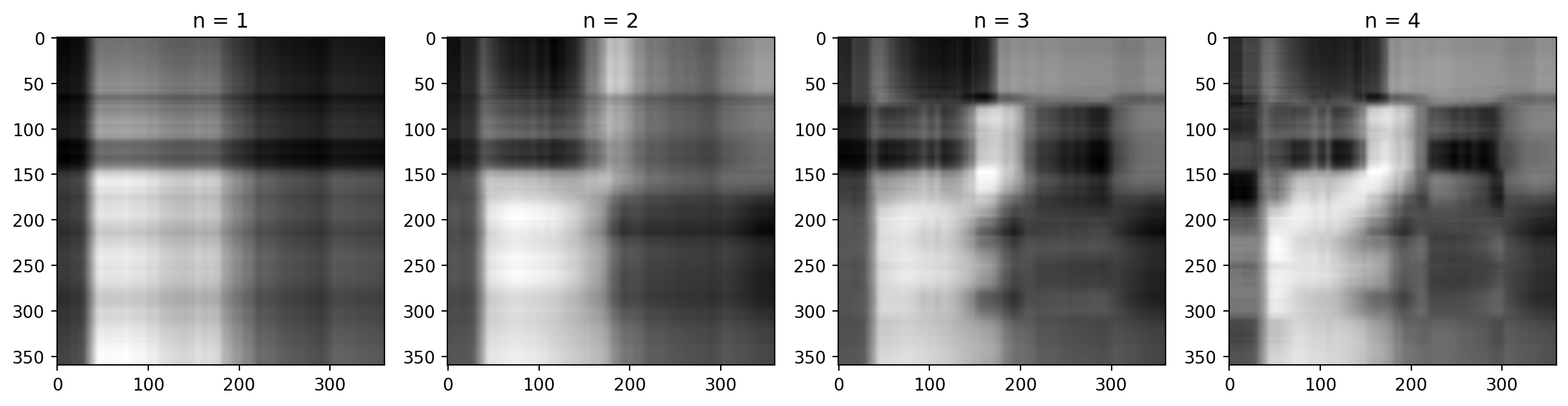
The data from these first two rows of the \(V^T\) matrix, after multiplication by the singular values and rotated by the columns of the U matrix:

A reminder:

\[ \mathbf A = \mathbf{USV^\mathsf{T}} = \sigma_1 u_1 v_1^\mathsf{T} + \dots + \sigma_r u_r v_r^\mathsf{T} \]

SVD on images

Motivation: a cat

Dimensions of the decomposition

What are the dimensions of the decompositions for an image?

Code

U, S, Vt = np.linalg.svd(image, full_matrices=False)
print(f'The shape of U is {U.shape}, the shape of S is {S.shape}, the shape of V is {Vt.shape}')

The shape of U is (360, 360), the shape of S is (360,), the shape of V is (360, 360)

pause

Left singular values, corresponding to U, are the eigenvalues of \(AA^T\). For an image, \(AA^T\) is the covariance matrix of the rows of \(A\).

Right singular values are the eigenvalues of \(A^{T}A\). For an image, \(A^TA\) is the covariance matrix of the columns of \(A\).

Simple example

Reconstructing our matrix

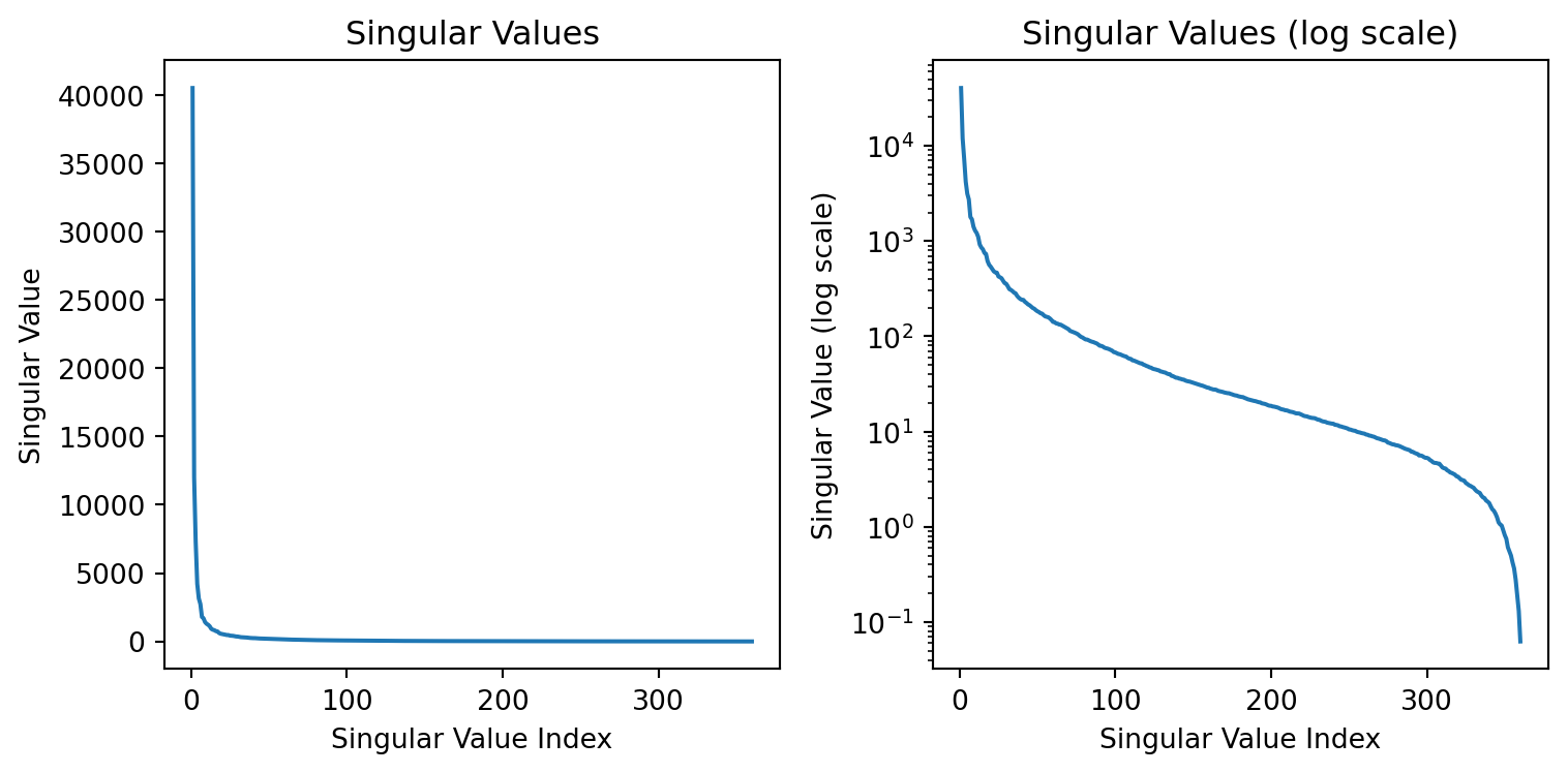
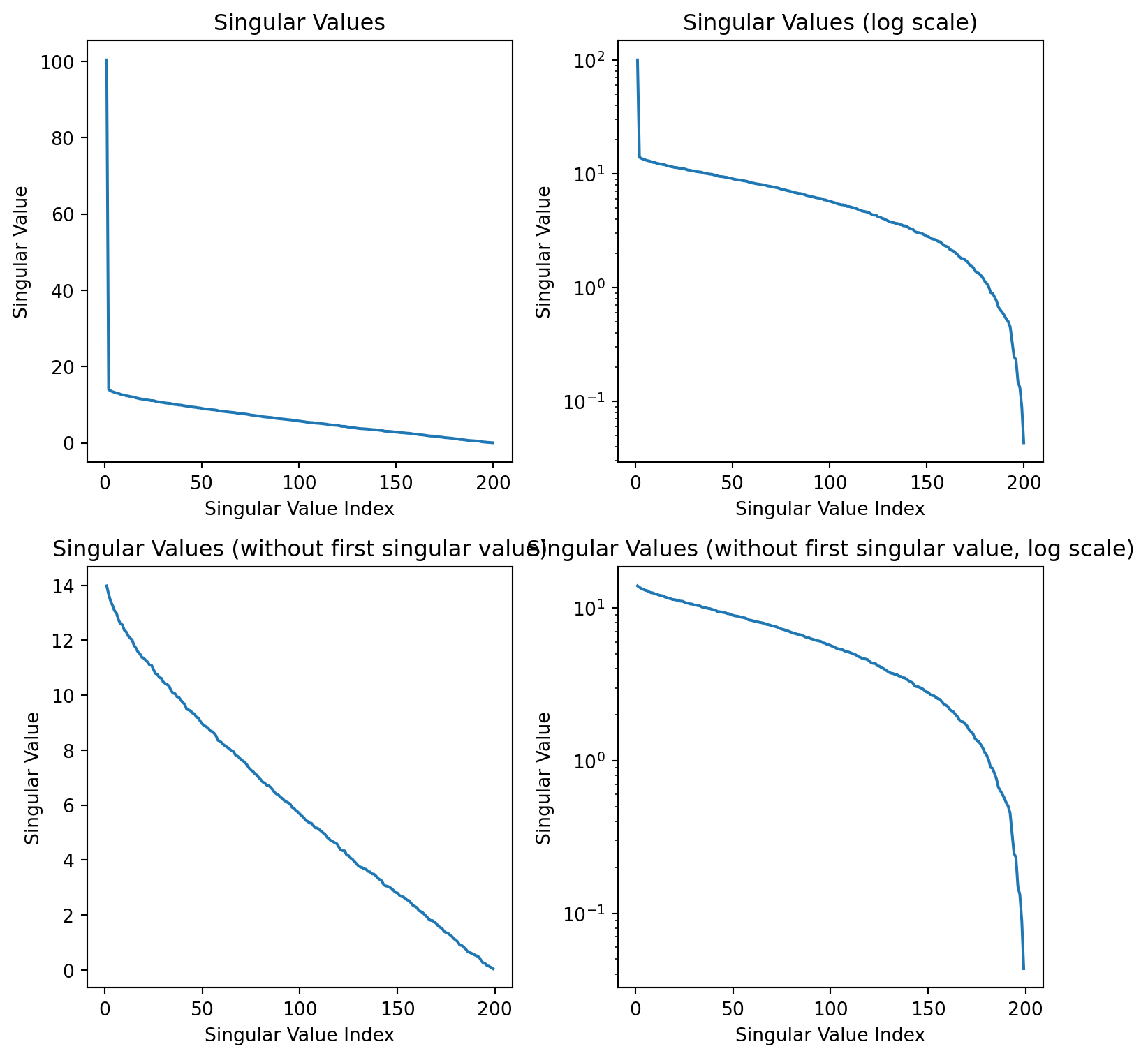
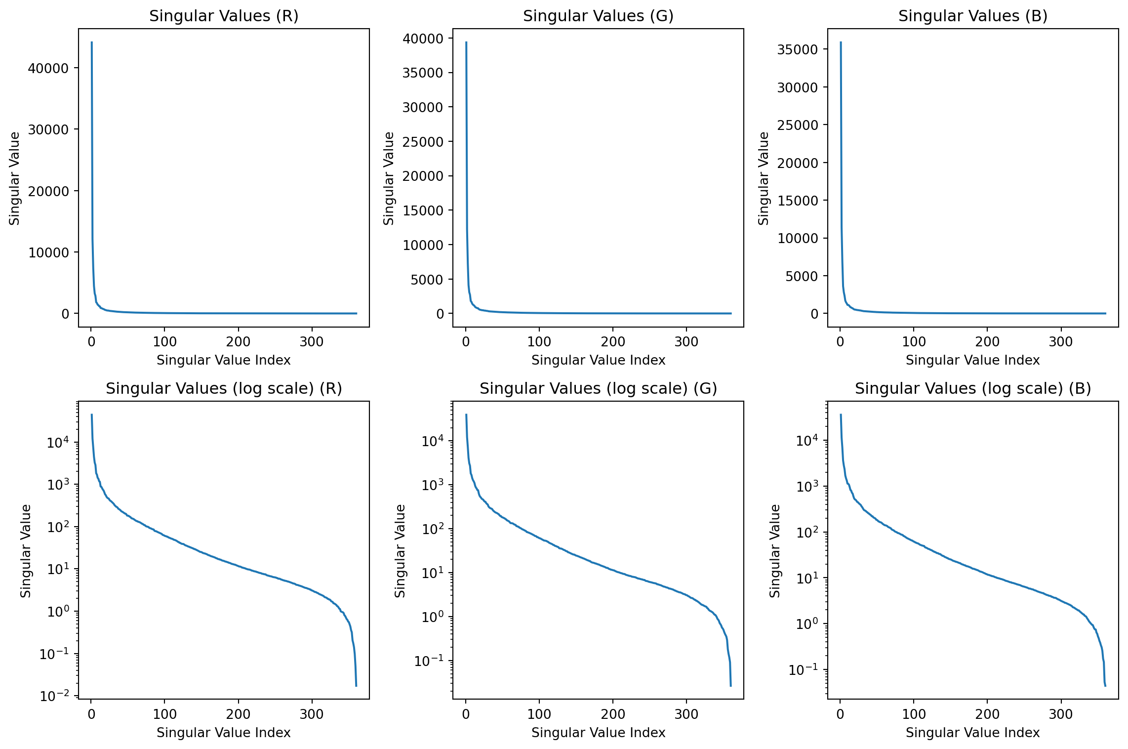
How much of the variance is captured by the first two components?

The variance captured by the each component is the sum of the squares of the singular values divided by the sum of the squares of all the singular values.

Back to the cat

First Singular Value

Second Singular Value

Third Singular Value

Adding them up

Color images

Code

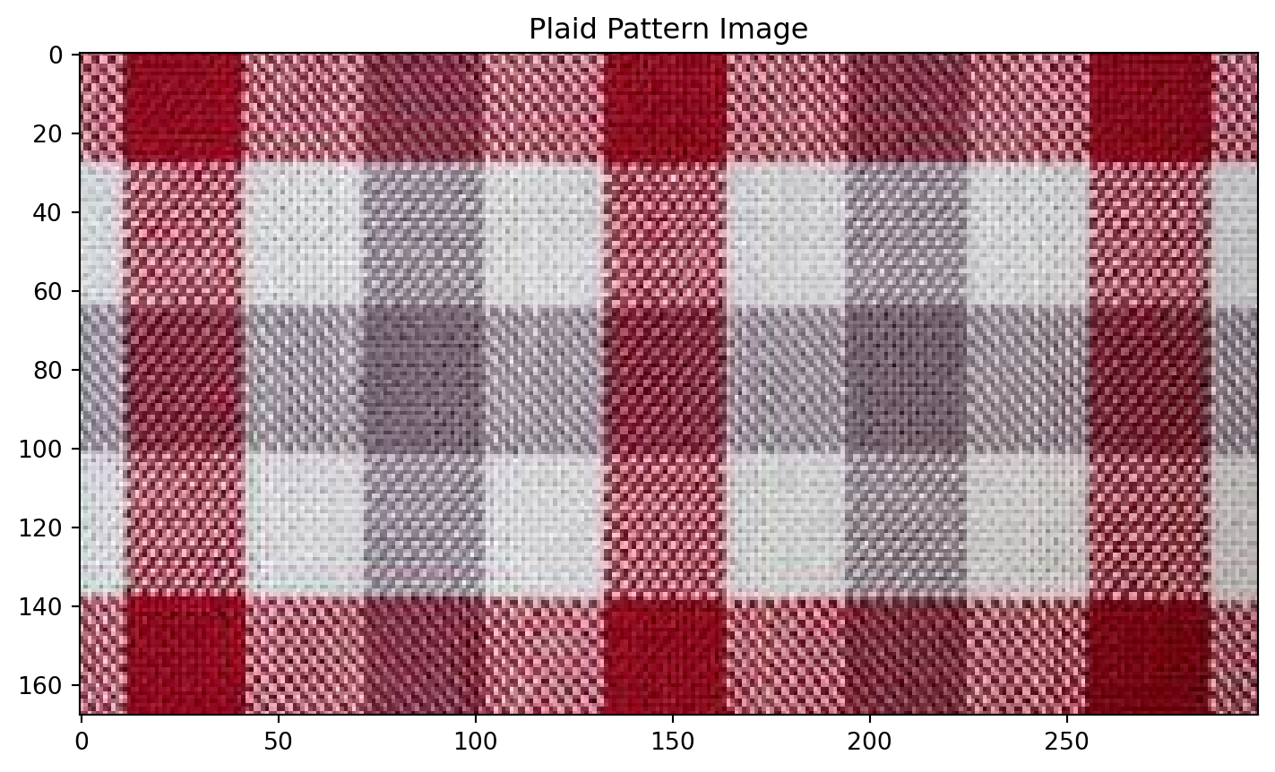
# SVD for each channel
U_R, S_R, Vt_R = np.linalg.svd(R, full_matrices=False)
U_G, S_G, Vt_G = np.linalg.svd(G, full_matrices=False)
U_B, S_B, Vt_B = np.linalg.svd(B, full_matrices=False)

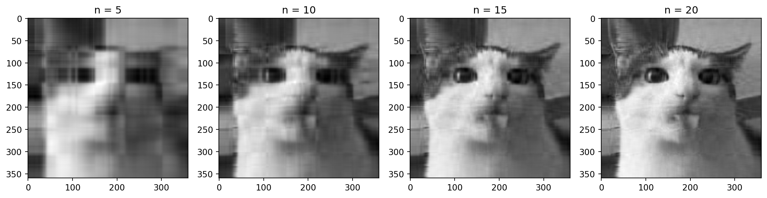
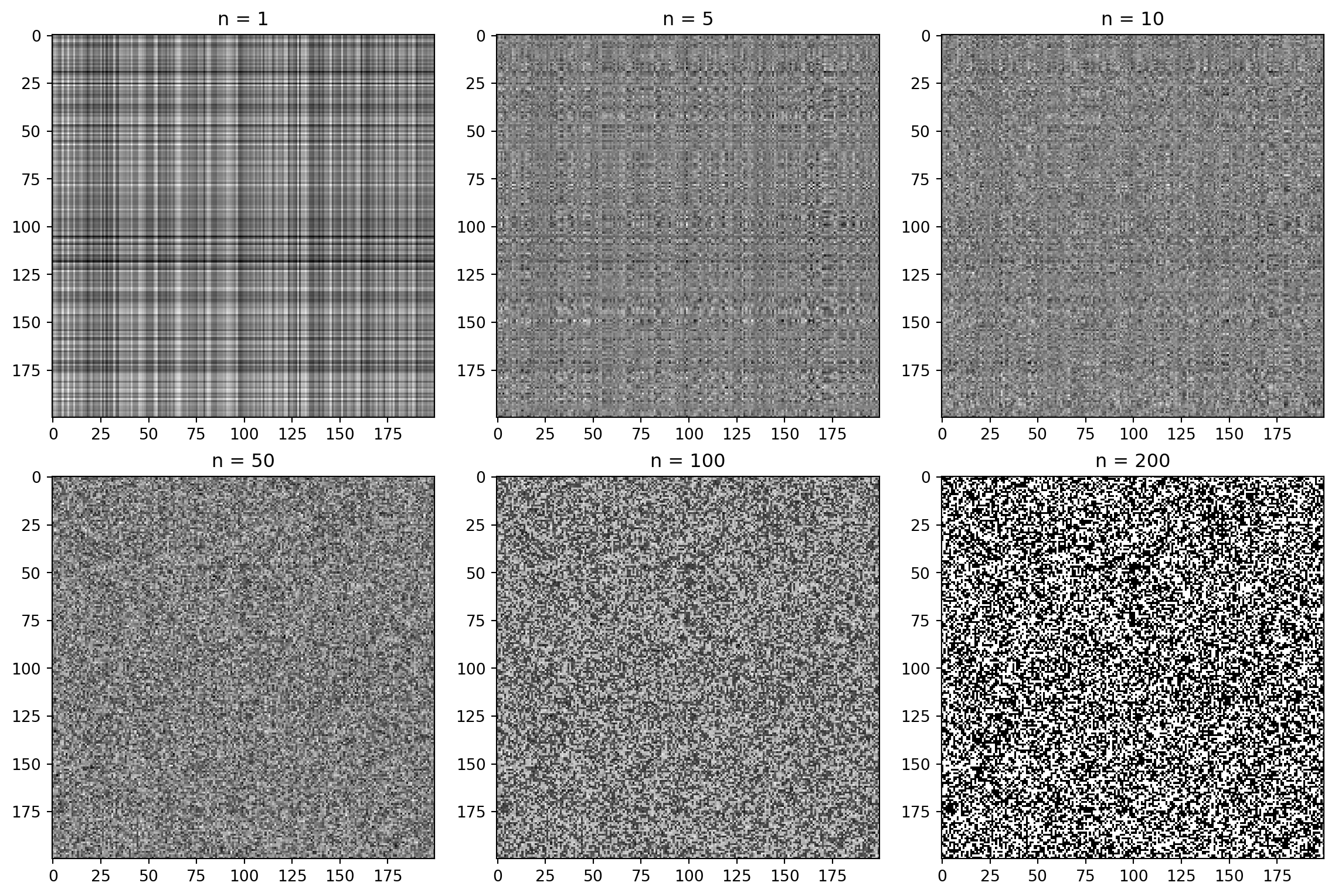
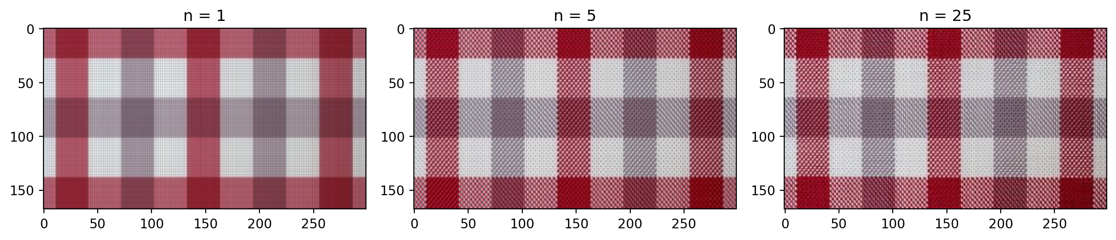
n = 50  # rank approximation parameter
R_compressed = np.matrix(U_R[:, :n]) * np.diag(S_R[:n]) * np.matrix(Vt_R[:n, :])
G_compressed = np.matrix(U_G[:, :n]) * np.diag(S_G[:n]) * np.matrix(Vt_G[:n, :])
B_compressed = np.matrix(U_B[:, :n]) * np.diag(S_B[:n]) * np.matrix(Vt_B[:n, :])

# Combining the compressed channels
compressed_image = cv2.merge([np.clip(R_compressed, 1, 255), np.clip(G_compressed, 1, 255), np.clip(B_compressed, 1, 255)])
compressed_image = compressed_image.astype(np.uint8)
plt.imshow(compressed_image)
plt.title('n = %s' % n)
plt.show()

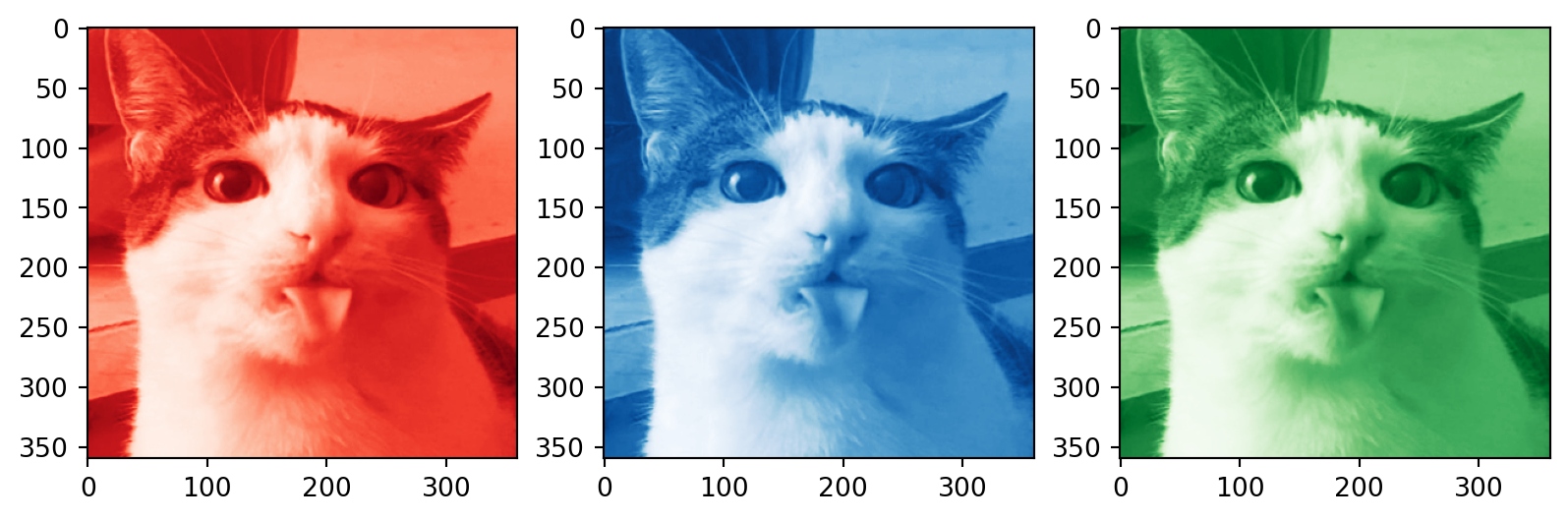
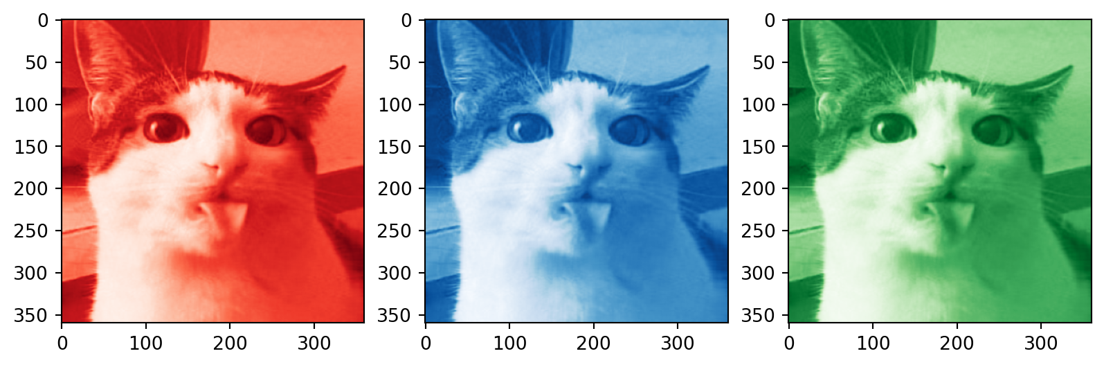
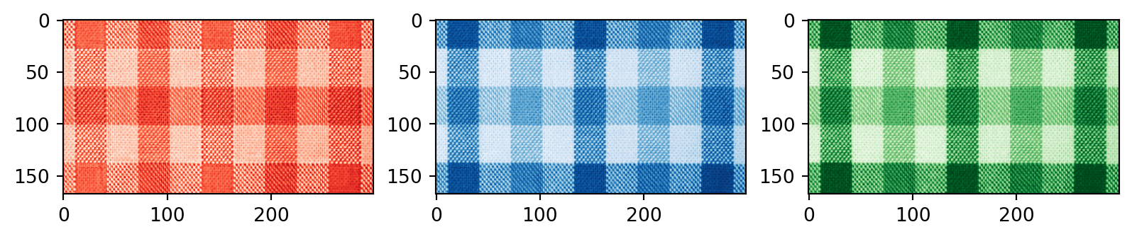
# Plotting the compressed RGB channels
plt.subplot(1, 3, 1)
plt.imshow(R_compressed, cmap='Reds_r')
plt.subplot(1, 3, 2)
plt.imshow(B_compressed, cmap='Blues_r')
plt.subplot(1, 3, 3)
plt.imshow(G_compressed, cmap='Greens_r')
plt.show()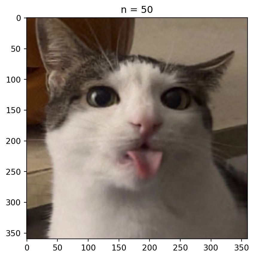

How many singular values to keep?

Different sorts of images

Just plain noise:

Code

noise = np.random.randint(0,2,size=(200,200))
plt.imshow(noise, cmap='gray')

pause

Plaid shirt

pause

Singular values

Individual components

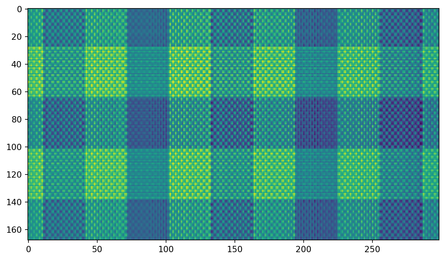
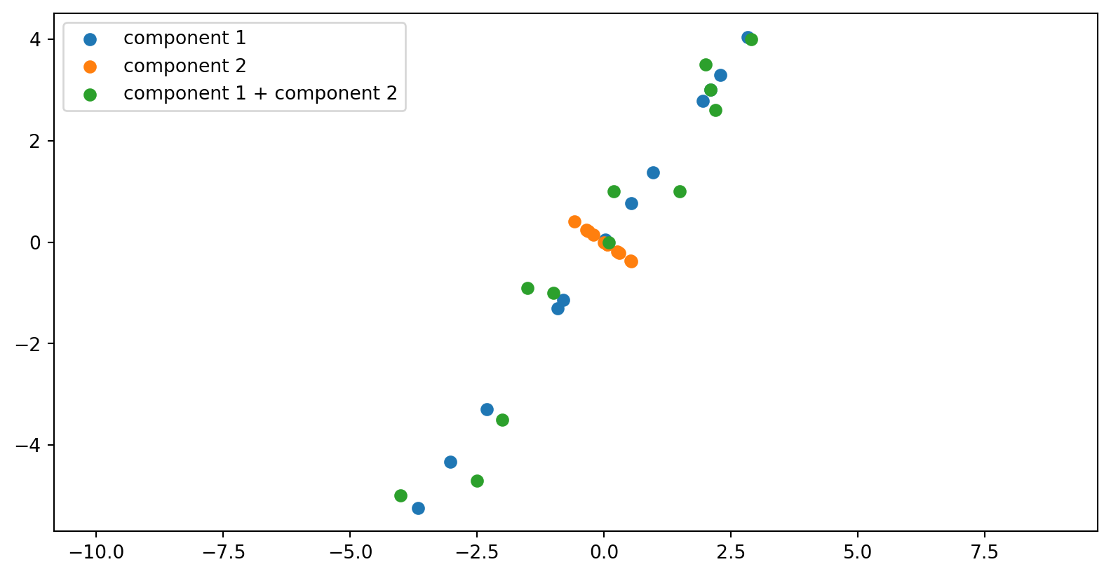
First component:

Second component:

Using “PCA” from sklearn

This is just an easier way to implement taking these first few components…

Code

from sklearn.decomposition import PCA
pca = PCA(n_components=2)
pca.fit(R) # fit the model -- compute the matrices
transformed = pca.transform(R) # transform the data
print(f'The shape of the image is {R.shape}, and the shape of the compressed image is {transformed.shape}')
plt.imshow(transformed.T)

The shape of the image is (168, 299), and the shape of the compressed image is (168, 2)

Code

plt.imshow(pca.inverse_transform(transformed))

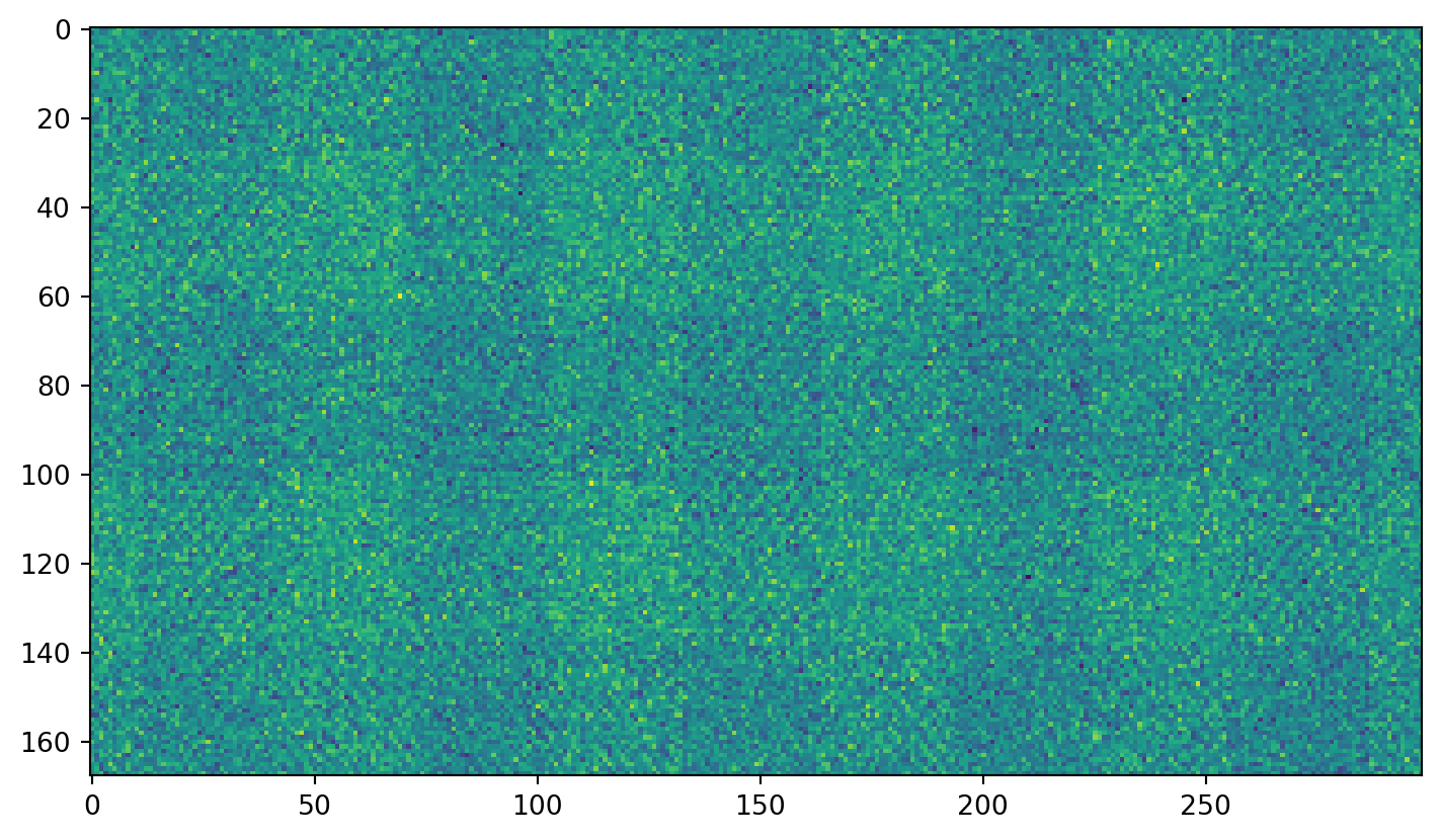
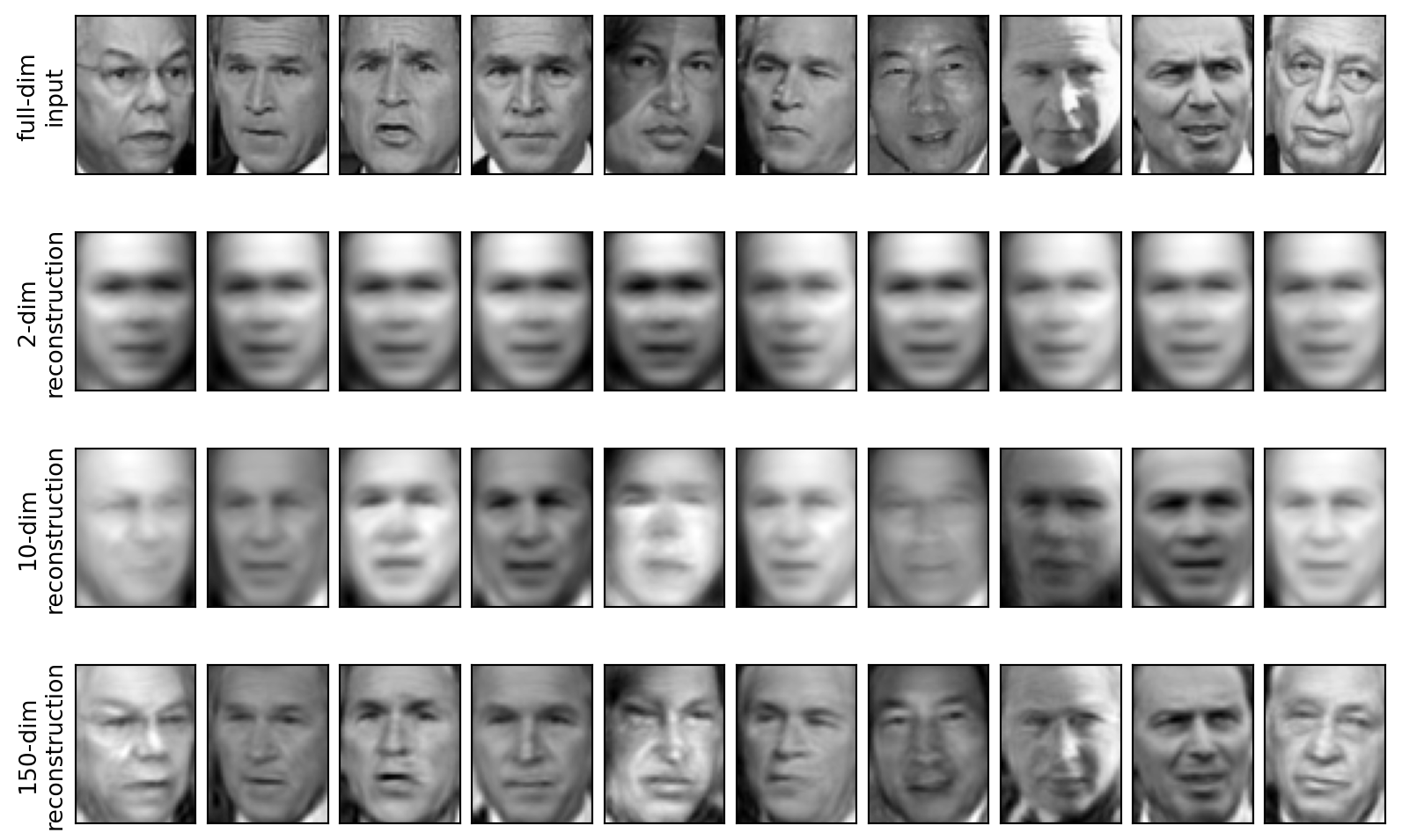
Try adding noise…

Code

alpha = 10
R_noisy = R + np.random.normal(0, 10, R.shape)*alpha
plt.imshow(R_noisy)

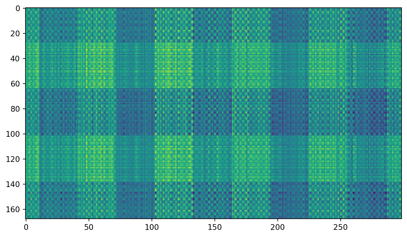
Now clean it up with PCA:

Code

pca = PCA(n_components=2)
pca.fit(R_noisy)
plt.imshow(pca.inverse_transform(pca.transform(R_noisy)))

SVD in higher dimensions

Faces

Code

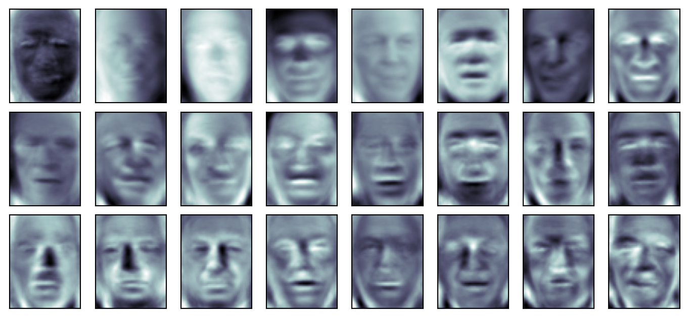
from sklearn.datasets import fetch_lfw_people
faces = fetch_lfw_people(min_faces_per_person=60)


# display a few of the faces, along with their names
fig, ax = plt.subplots(3, 4)
for i, axi in enumerate(ax.flat):
    axi.imshow(faces.images[i], cmap='bone')
    axi.set(xticks=[], yticks=[],
            xlabel=faces.target_names[faces.target[i]]) 

print(f'The shape of the faces dataset is {faces.images.shape}')

The shape of the faces dataset is (1348, 62, 47)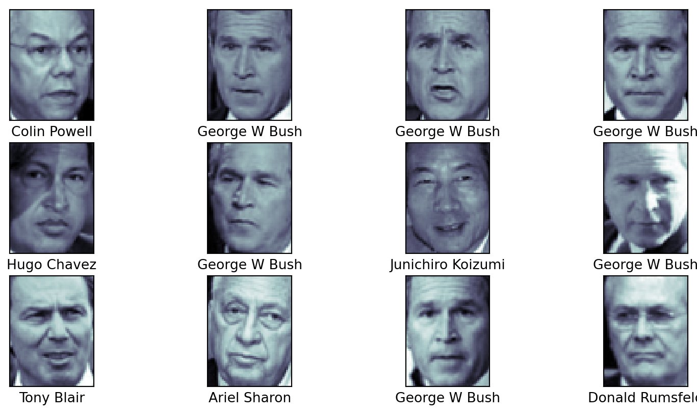

pause

PCA on faces

Code

pca = PCA(150, svd_solver='randomized', random_state=42)
pca_small = PCA(10, svd_solver='randomized', random_state=42)
pca_very_small = PCA(2, svd_solver='randomized', random_state=42)
pca.fit(faces.data)
pca_small.fit(faces.data)
pca_very_small.fit(faces.data)

PCA(n_components=2, random_state=42, svd_solver='randomized')

In a Jupyter environment, please rerun this cell to show the HTML representation or trust the notebook.
On GitHub, the HTML representation is unable to render, please try loading this page with nbviewer.org.

Reconstructions

Really cool demo of SVD image compression: https://timbaumann.info/svd-image-compression-demo/

Now you

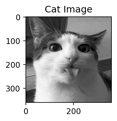
Code up your own image compression using SVD and show the left and right singular vectors, the singular values, and the reconstructed images.

Share with the class!