Ch4 Lecture 2
More Least Squares
Extending the normal equations to multiple predictors; geometry and a worked example.
Normal equations for multiple predictors
When we have multiple predictors, \(\mathbf{A}\) is a matrix
. . .
Each column corresponds to a predictor variable.
. . .
\(\mathbf{x}\) is a column vector of the coefficients we are trying to find, one per predictor.
. . .
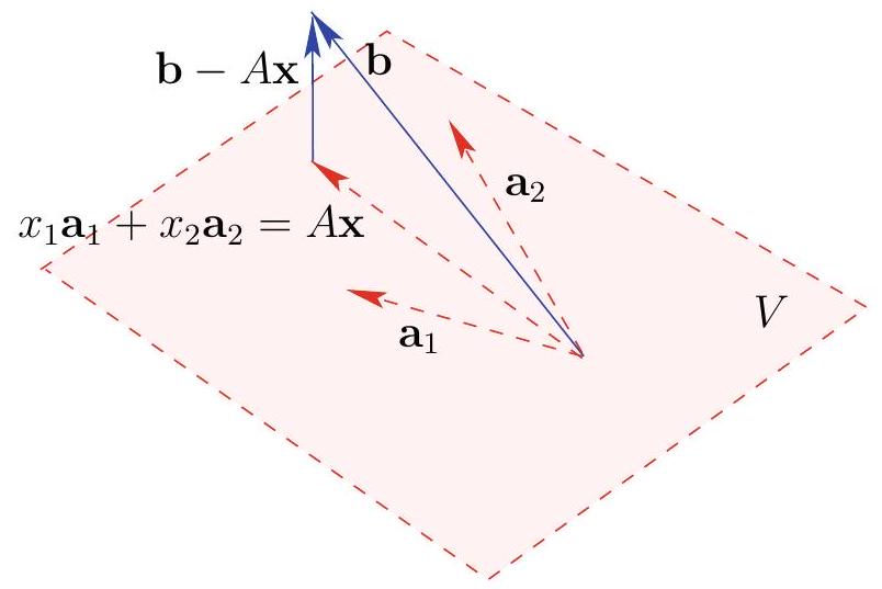
What do the normal equations tell us? We can break them apart into one equation corresponding to each column of \(\mathbf{A}\).
. . .
\[ \begin{aligned} \mathbf{A}^T \mathbf{A} \mathbf{x} &=\mathbf{A}^T \mathbf{b} \\ \text{becomes} \\ \mathbf{a}_i \cdot \mathbf{A} \mathbf{x} &=\mathbf{a}_i \cdot \mathbf{b} \text{ for every } i \\ \mathbf{a}_i \cdot (\mathbf{b}-\mathbf{A}\mathbf{x})&=0 \text{ for every } i \end{aligned} \]
. . .
We need to find \(\mathbf{x}\) such that the residuals are orthogonal to every column of \(\mathbf{A}\).
. . .
Figure
Example
We have two predictors \(a_1\) and \(a_2\) and a response variable \(b\). We have the following data:
| \(x_1\) | \(x_2\) | \(y\) |
|---|---|---|
| 2 | 1 | 0 |
| 1 | 1 | 0 |
| 2 | 1 | 2 |
. . .
We are hoping to find a linear relationship of the form \(\beta_1 x_1 + \beta_2 x_2 = y\) for some values of \(\beta_1\) and \(\beta_2\).
. . .
This would bring us the following system of equations:
\[ \begin{aligned} 2 \beta_{1}+\beta_{2} & =0 \\ \beta_{1}+\beta_{2} & =0 \\ 2 \beta_{1}+\beta_{2} & =2 . \end{aligned} \]
. . .
Obviously inconsistent! (\(2 \beta_{1}+\beta_{2}\) cannot equal both 0 and 2.)
. . .
Find the least squares solution using the normal equations:
. . .
Matrix form
Change variable names: the \(\beta\)s are now \(\mathbf{x}\), the predictor columns are \(\mathbf{A}\), and the \(y\)s are now \(\mathbf{b}\).
\[ \mathbf{A}=\left[\begin{array}{ll} 2 & 1 \\ 1 & 1 \\ 2 & 1 \end{array}\right], \text { and } \mathbf{b}=\left[\begin{array}{l} 0 \\ 0 \\ 2 \end{array}\right] \]
. . .
Residuals are \(\mathbf{b}-\mathbf{A} \mathbf{x}\).
Normal equations are \(\mathbf{A}^T \mathbf{A} \mathbf{x}=\mathbf{A}^T \mathbf{b}\).
. . .
Solve via \(\mathbf{A}^T\mathbf{A}\)
\[ \mathbf{A}^T \mathbf{A}=\left[\begin{array}{lll} 2 & 1 & 2 \\ 1 & 1 & 1 \end{array}\right]\left[\begin{array}{ll} 2 & 1 \\ 1 & 1 \\ 2 & 1 \end{array}\right]=\left[\begin{array}{ll} 9 & 5 \\ 5 & 3 \end{array}\right] \]
with inverse \[ \left(\mathbf{A}^T \mathbf{A}\right)^{-1}=\left[\begin{array}{ll} 9 & 5 \\ 5 & 3 \end{array}\right]^{-1}=\frac{1}{2}\left[\begin{array}{rr} 3 & -5 \\ -5 & 9 \end{array}\right] \]
. . .
\[ \mathbf{A}^T \mathbf{b}=\left[\begin{array}{lll} 2 & 1 & 2 \\ 1 & 1 & 1 \end{array}\right]\left[\begin{array}{l} 0 \\ 0 \\ 2 \end{array}\right]=\left[\begin{array}{l} 4 \\ 2 \end{array}\right] \]
Least Squares Solution
\[ \mathbf{x}=\left(\mathbf{A}^T \mathbf{A}\right)^{-1} \mathbf{A}^T \mathbf{b}=\frac{1}{2}\left[\begin{array}{rr} 3 & -5 \\ -5 & 9 \end{array}\right]\left[\begin{array}{l} 4 \\ 2 \end{array}\right]=\left[\begin{array}{r} 1 \\ -1 \end{array}\right] \]
. . .
Back in our original variables, this means the best fit estimate for \(\beta_1\) is 1 and the best \(\beta_2\) is -1.
. . .
Skills
- Write the normal equations \(\mathbf{A}^T \mathbf{A} \mathbf{x} = \mathbf{A}^T \mathbf{b}\) for a given design matrix \(\mathbf{A}\) and response \(\mathbf{b}\).
- Interpret the equations as “residuals orthogonal to every column of \(\mathbf{A}\).”
- Find the least-squares solution by computing \(\mathbf{A}^T \mathbf{A}\), its inverse, and \(\mathbf{A}^T \mathbf{b}\) (when invertible).
Orthogonal and Orthonormal Sets
The set of vectors \(\mathbf{v}_{1}, \mathbf{v}_{2}, \ldots, \mathbf{v}_{n}\) is an orthogonal set if \(\mathbf{v}_{i} \cdot \mathbf{v}_{j}=0\) whenever \(i \neq j\).
If, in addition, each vector has unit length, i.e., \(\mathbf{v}_{i} \cdot \mathbf{v}_{i}=1\), then the set of vectors is orthonormal .
Orthogonal Coordinates Theorem
If \(\mathbf{v}_{1}, \mathbf{v}_{2}, \ldots, \mathbf{v}_{n}\) are nonzero and orthogonal, and
\(\mathbf{v} \in \operatorname{span}\left\{\mathbf{v}_{1}, \mathbf{v}_{2}, \ldots, \mathbf{v}_{n}\right\}\),
\(\mathbf{v}\) can be expressed uniquely (up to order) as a linear combination of \(\mathbf{v}_{1}, \mathbf{v}_{2}, \ldots, \mathbf{v}_{n}\), namely
\[ \mathbf{v}=\frac{\mathbf{v}_{1} \cdot \mathbf{v}}{\mathbf{v}_{1} \cdot \mathbf{v}_{1}} \mathbf{v}_{1}+\frac{\mathbf{v}_{2} \cdot \mathbf{v}}{\mathbf{v}_{2} \cdot \mathbf{v}_{2}} \mathbf{v}_{2}+\cdots+\frac{\mathbf{v}_{n} \cdot \mathbf{v}}{\mathbf{v}_{n} \cdot \mathbf{v}_{n}} \mathbf{v}_{n} \]
Proof
Since \(\mathbf{v} \in \operatorname{span}\left\{\mathbf{v}_{1}, \mathbf{v}_{2}, \ldots, \mathbf{v}_{n}\right\}\),
we can write \(\mathbf{v}\) as a linear combination of the \(\mathbf{v}_{i}\) ’s:
\[ \mathbf{v}=c_{1} \mathbf{v}_{1}+c_{2} \mathbf{v}_{2}+\cdots+c_{n} \mathbf{v}_{n} \]
. . .
Now take the inner product of both sides with \(\mathbf{v}_{k}\):
. . .
Since \(\mathbf{v}_{k} \cdot \mathbf{v}_{j}=0\) if \(j \neq k\),
\[ \begin{aligned} \mathbf{v}_{k} \cdot \mathbf{v} & =\mathbf{v}_{k} \cdot\left(c_{1} \mathbf{v}_{1}+c_{2} \mathbf{v}_{2}+\ldots \cdots+c_{n} \mathbf{v}_{n}\right) \\ & =c_{1} \mathbf{v}_{k} \cdot \mathbf{v}_{1}+c_{2} \mathbf{v}_{k} \cdot \mathbf{v}_{2}+\cdots+c_{n} \mathbf{v}_{k} \cdot \mathbf{v}_{n}=c_{k} \mathbf{v}_{k} \cdot \mathbf{v}_{k} \end{aligned} \]
. . .
Since \(\mathbf{v}_{k} \neq 0\), \(\left\|\mathbf{v}_{k}\right\|^{2}=\mathbf{v}_{k} \cdot \mathbf{v}_{k} \neq 0\) so we can divide:
\[ c_{k}=\frac{\mathbf{v}_{k} \cdot \mathbf{v}}{\mathbf{v}_{k} \cdot \mathbf{v}_{k}} \]
. . .
Any linear combination of an orthogonal set of nonzero vectors is the sum of its projections in the direction of each vector in the set.
Orthogonal matrix (definition)
A square real matrix \(Q\) is called orthogonal if \(Q^{T}=Q^{-1}\).
A square matrix \(U\) is called unitary if \(U^{*}=U^{-1}\).
Example
Show that the matrix \(R(\theta)=\left[\begin{array}{rr}\cos \theta & -\sin \theta \\ \sin \theta & \cos \theta\end{array}\right]\) is orthogonal.
. . .
\[ \begin{aligned} R(\theta)^{T} R(\theta) & =\left(\left[\begin{array}{cc} \cos \theta & -\sin \theta \\ \sin \theta & \cos \theta \end{array}\right]\right)^{T}\left[\begin{array}{cc} \cos \theta & -\sin \theta \\ \sin \theta & \cos \theta \end{array}\right] \\ & =\left[\begin{array}{cc} \cos \theta \sin \theta \\ -\sin \theta \cos \theta \end{array}\right]\left[\begin{array}{cc} \cos \theta-\sin \theta \\ \sin \theta & \cos \theta \end{array}\right] \\ & =\left[\begin{array}{cc} \cos ^{2} \theta+\sin ^{2} \theta & \cos \theta \sin \theta-\sin \theta \cos \theta \\ -\cos \theta \sin \theta+\sin \theta \cos \theta & \sin ^{2} \theta+\cos ^{2} \theta \end{array}\right]=\left[\begin{array}{ll} 1 & 0 \\ 0 & 1 \end{array}\right], \end{aligned} \]
Orthogonal matrix from orthonormal columns
Suppose \(\mathbf{u}_{1}, \mathbf{u}_{2}, \ldots, \mathbf{u}_{n}\) is an orthonormal basis of \(\mathbb{R}^{n}\)
. . .
Make these the column vectors of \(\mathbf{A}\): \(\mathbf{A}=\left[\mathbf{u}_{1}, \mathbf{u}_{2}, \ldots, \mathbf{u}_{n}\right]\)
. . .
Because the \(\mathbf{u}_{i}\) are orthonormal, \(\mathbf{u}_{i}^{T} \mathbf{u}_{j}=\delta_{i j}\)
. . .
Use this to calculate \(A^{T} A\).
- Its \((i,j)\)-th entry is \(\mathbf{u}_i^T \mathbf{u}_j\).
- So \(A^T A = [\delta_{ij}] = I\).
- Therefore \(A^T = A^{-1}\).
. . .
Rigidity of orthogonal (and unitary) matrices
Suppose we have two vectors \(\mathbf{x}\) and \(\mathbf{y}\) in \(\mathbb{R}^n\), with an angle \(\phi\) between them.
. . .
What happens if we apply the rotation matrix \(R(\theta)\) to both vectors? (Show by drawing.)
\[ R(\theta) = \left[\begin{array}{cc} \cos \theta & -\sin \theta \\ \sin \theta & \cos \theta \end{array}\right] \]
. . .
The length of each vector stays the same, and the angle between them also remains the same.
. . .
The rotation matrix preserves vector lengths and angles between vectors.
\[ R(\theta)\mathbf{x}\cdot R(\theta)\mathbf{y}=\mathbf{x} \cdot \mathbf{y} \]
Rigidity of orthogonal (and unitary) matrices (continued)
This is true in general for orthogonal matrices. If \(Q\) is orthogonal, then
\[ Q \mathbf{x} \cdot Q \mathbf{y}=(Q \mathbf{x})^{T} Q \mathbf{y}=\mathbf{x}^{T} Q^{T} Q \mathbf{y}=\mathbf{x}^{T} \mathbf{y}=\mathbf{x} \cdot \mathbf{y} \]
also,
\[ \|Q \mathbf{x}\|^{2}=Q \mathbf{x} \cdot Q \mathbf{x}=(Q \mathbf{x})^{T} Q \mathbf{x}=\mathbf{x}^{T} Q^{T} Q \mathbf{x}=\mathbf{x}^{T} \mathbf{x}=\|\mathbf{x}\|^{2} \]
. . .
Skills
- State the definitions of orthogonal set, orthonormal set, and orthogonal matrix.
- Use the orthogonal coordinates formula to write a vector as a linear combination of orthogonal basis vectors.
- Explain why orthogonal matrices preserve dot products and lengths.
Finding orthogonal bases
Gram-Schmidt Algorithm
Let \(\mathbf{w}_{1}, \mathbf{w}_{2}, \ldots, \mathbf{w}_{n}\) be linearly independent vectors in a standard space.
. . .
Define vectors \(\mathbf{v}_{1}, \mathbf{v}_{2}, \ldots, \mathbf{v}_{n}\) recursively:
Take each \(\mathbf{w}_{k}\) and subtract off the projection of \(\mathbf{w}_{k}\) onto each of the previous vectors \(\mathbf{v}_{1}, \mathbf{v}_{2}, \ldots, \mathbf{v}_{k-1}\)
. . .
\[ \mathbf{v}_{k}=\mathbf{w}_{k}-\frac{\mathbf{v}_{1} \cdot \mathbf{w}_{k}}{\mathbf{v}_{1} \cdot \mathbf{v}_{1}} \mathbf{v}_{1}-\frac{\mathbf{v}_{2} \cdot \mathbf{w}_{k}}{\mathbf{v}_{2} \cdot \mathbf{v}_{2}} \mathbf{v}_{2}-\cdots-\frac{\mathbf{v}_{k-1} \cdot \mathbf{w}_{k}}{\mathbf{v}_{k-1} \cdot \mathbf{v}_{k-1}} \mathbf{v}_{k-1}, \quad k=1, \ldots, n \]
. . .
Gram–Schmidt: key facts
\[ \mathbf{v}_{k}=\mathbf{w}_{k}-\frac{\mathbf{v}_{1} \cdot \mathbf{w}_{k}}{\mathbf{v}_{1} \cdot \mathbf{v}_{1}} \mathbf{v}_{1}-\frac{\mathbf{v}_{2} \cdot \mathbf{w}_{k}}{\mathbf{v}_{2} \cdot \mathbf{v}_{2}} \mathbf{v}_{2}-\cdots-\frac{\mathbf{v}_{k-1} \cdot \mathbf{w}_{k}}{\mathbf{v}_{k-1} \cdot \mathbf{v}_{k-1}} \mathbf{v}_{k-1}, \quad k=1, \ldots, n \]
. . .
Then:
- The vectors \(\mathbf{v}_{1}, \mathbf{v}_{2}, \ldots, \mathbf{v}_{k}\) form an orthogonal set.
- For each \(k=1, \ldots, n\), \(\operatorname{span}\left\{\mathbf{w}_{1}, \ldots, \mathbf{w}_{k}\right\}=\operatorname{span}\left\{\mathbf{v}_{1}, \ldots, \mathbf{v}_{k}\right\}\).
. . .
\[ \operatorname{span}\left\{\mathbf{w}_{1}, \mathbf{w}_{2}, \ldots, \mathbf{w}_{k}\right\}=\operatorname{span}\left\{\mathbf{v}_{1}, \mathbf{v}_{2}, \ldots, \mathbf{v}_{k}\right\} \]
Example
Let \(V=\mathcal{C}(A)\) with the standard inner product and compute an orthonormal basis of \(V\), where
\[ A=\left[\begin{array}{rrrr} 1 & 2 & 0 & -1 \\ 1 & -1 & 3 & 2 \\ 1 & -1 & 3 & 2 \\ -1 & 1 & -3 & 1 \end{array}\right] \]
. . .
RREF of \(A\) is:
\[ R=\left[\begin{array}{rrrr} 1 & 0 & 2 & 0 \\ 0 & 1 & -1 & 0 \\ 0 & 0 & 0 & 1 \\ 0 & 0 & 0 & 0 \end{array}\right] \]
. . .
The independent columns are columns 1, 2, and 4.
. . .
So let these be our \(\mathbf{w}_{1}, \mathbf{w}_{2}, \mathbf{w}_{3}\).
. . .
Gram–Schmidt steps
Step 1: \(\mathbf{v}_{1}=\mathbf{w}_{1}=(1,1,1,-1)\)
. . .
Step 2: \(\mathbf{v}_{2}=\mathbf{w}_{2}-\frac{\mathbf{v}_{1} \cdot \mathbf{w}_{2}}{\mathbf{v}_{1} \cdot \mathbf{v}_{1}} \mathbf{v}_{1}\)
. . .
\(=(2,-1,-1,1)-\frac{-1}{4}(1,1,1,-1)=\frac{1}{4}(9,-3,-3,3)\)
. . .
Step 3: \(\mathbf{v}_{3}=\mathbf{w}_{3}-\frac{\mathbf{v}_{1} \cdot \mathbf{w}_{3}}{\mathbf{v}_{1} \cdot \mathbf{v}_{1}} \mathbf{v}_{1}-\frac{\mathbf{v}_{2} \cdot \mathbf{w}_{3}}{\mathbf{v}_{2} \cdot \mathbf{v}_{2}} \mathbf{v}_{2}\)
. . .
\(=(-1,2,2,1)-\frac{2}{4}(1,1,1,-1)-\frac{-18}{108}(9,-3,-3,3)=(0,1,1,2)\)
Finding orthonormal basis
Now we need to normalize these vectors to get an orthonormal basis.
. . .
\(\mathbf{u}_{1}=\frac{1}{\|\mathbf{v}_{1}\|} \mathbf{v}_{1}=\frac{1}{2}(1,1,1,-1)\)
. . .
\(\mathbf{u}_{2}=\frac{1}{\|\mathbf{v}_{2}\|} \mathbf{v}_{2}=\frac{1}{\sqrt{108}}(9,-3,-3,3)\)
. . .
(Continue similarly for \(\mathbf{u}_3\), etc.)
. . .
Skills
- Run the Gram–Schmidt algorithm on a set of linearly independent vectors to get an orthogonal set.
- Normalize to obtain an orthonormal basis.
- Identify which columns of a matrix are linearly independent (e.g. via RREF) before applying Gram–Schmidt.
QR Factorization
Every full-column-rank matrix factors as \(A=QR\); use it to solve linear systems and least squares more stably.
If \(A\) is an \(m \times n\) full-column-rank matrix, then \(A=Q R\), where the columns of the \(m \times n\) matrix \(Q\) are orthonormal vectors and the \(n \times n\) matrix \(R\) is upper triangular with nonzero diagonal entries.
. . .
Why we care
- Solve linear systems \(A\mathbf{x}=\mathbf{b}\) via \(R\mathbf{x}=Q^T\mathbf{b}\) (often more stable than Gauss–Jordan).
- Solve least squares \(\mathbf{A}\mathbf{x}\approx\mathbf{b}\) using QR (same idea; we’ll see how).
. . .
How to find \(Q\) and \(R\)
- Start with the columns of \(A\), \(A=\left[\mathbf{w}_{1}, \mathbf{w}_{2}, \mathbf{w}_{3}\right]\). (Assume they are linearly independent.)
- Do Gram–Schmidt on the columns of \(A\):
. . .
\[ \begin{aligned} & \mathbf{v}_{1}=\mathbf{w}_{1} \\ & \mathbf{v}_{2}=\mathbf{w}_{2}-\frac{\mathbf{v}_{1} \cdot \mathbf{w}_{2}}{\mathbf{v}_{1} \cdot \mathbf{v}_{1}} \mathbf{v}_{1} \\ & \mathbf{v}_{3}=\mathbf{w}_{3}-\frac{\mathbf{v}_{1} \cdot \mathbf{w}_{3}}{\mathbf{v}_{1} \cdot \mathbf{v}_{1}} \mathbf{v}_{1}-\frac{\mathbf{v}_{2} \cdot \mathbf{w}_{3}}{\mathbf{v}_{2} \cdot \mathbf{v}_{2}} \mathbf{v}_{2} . \end{aligned} \]
. . .
- Solve these equations for \(\mathbf{w}_{1}, \mathbf{w}_{2}, \mathbf{w}_{3}\):
. . .
\[ \begin{aligned} & \mathbf{w}_{1}=\mathbf{v}_{1} \\ & \mathbf{w}_{2}=\frac{\mathbf{v}_{1} \cdot \mathbf{w}_{2}}{\mathbf{v}_{1} \cdot \mathbf{v}_{1}} \mathbf{v}_{1}+\mathbf{v}_{2} \\ & \mathbf{w}_{3}=\frac{\mathbf{v}_{1} \cdot \mathbf{w}_{3}}{\mathbf{v}_{1} \cdot \mathbf{v}_{1}} \mathbf{v}_{1}+\frac{\mathbf{v}_{2} \cdot \mathbf{w}_{3}}{\mathbf{v}_{2} \cdot \mathbf{v}_{2}} \mathbf{v}_{2}+\mathbf{v}_{3} . \end{aligned} \]
. . .
Same relations, matrix form
\[ \begin{aligned} & \mathbf{w}_{1}=\mathbf{v}_{1} \\ & \mathbf{w}_{2}=\frac{\mathbf{v}_{1} \cdot \mathbf{w}_{2}}{\mathbf{v}_{1} \cdot \mathbf{v}_{1}} \mathbf{v}_{1}+\mathbf{v}_{2} \\ & \mathbf{w}_{3}=\frac{\mathbf{v}_{1} \cdot \mathbf{w}_{3}}{\mathbf{v}_{1} \cdot \mathbf{v}_{1}} \mathbf{v}_{1}+\frac{\mathbf{v}_{2} \cdot \mathbf{w}_{3}}{\mathbf{v}_{2} \cdot \mathbf{v}_{2}} \mathbf{v}_{2}+\mathbf{v}_{3} . \end{aligned} \]
In matrix form, these become:
. . .
\[ A=\left[\mathbf{w}_{1}, \mathbf{w}_{2}, \mathbf{w}_{3}\right]=\left[\mathbf{v}_{1}, \mathbf{v}_{2}, \mathbf{v}_{3}\right]\left[\begin{array}{ccc} 1 & \frac{\mathbf{v}_{1} \cdot \mathbf{w}_{2}}{\mathbf{v}_{1} \cdot \mathbf{v}_{1}} & \frac{\mathbf{v}_{1} \cdot \mathbf{w}_{3}}{\mathbf{v}_{1} \cdot \mathbf{v}_{1}} \\ 0 & 1 & \frac{\mathbf{v}_{2} \cdot \mathbf{w}_{3}}{\mathbf{v}_{2} \cdot \mathbf{v}_{2}} \\ 0 & 0 & 1 \end{array}\right] \]
Normalizing \(Q\)
We can normalize the columns of \(Q\) by dividing each column by its length.
. . .
Set \(\mathbf{q}_{j}=\mathbf{v}_{j} /\left\|\mathbf{v}_{j}\right\|\).
. . .
\[ \begin{aligned} A & =\left[\mathbf{q}_{1}, \mathbf{q}_{2}, \mathbf{q}_{3}\right]\left[\begin{array}{ccc} \left\|\mathbf{v}_{1}\right\| & 0 & 0 \\ 0 & \left\|\mathbf{v}_{2}\right\| & 0 \\ 0 & 0 & \left\|\mathbf{v}_{3}\right\| \end{array}\right]\left[\begin{array}{ccc} 1 & \frac{\mathbf{v}_{1} \cdot \mathbf{w}_{2}}{\mathbf{v}_{1} \cdot \mathbf{v}_{1}} & \frac{\mathbf{v}_{1} \cdot \mathbf{w}_{3}}{\mathbf{v}_{1} \cdot \mathbf{v}_{1}} \\ 0 & 1 & \frac{\mathbf{v}_{2} \cdot \mathbf{w}_{3}}{\mathbf{v}_{2}, \mathbf{v}_{2}} \\ 0 & 0 & 1 \end{array}\right] \end{aligned} \]
. . .
\[ \begin{aligned} & =\left[\mathbf{q}_{1}, \mathbf{q}_{2}, \mathbf{q}_{3}\right]\left[\begin{array}{ccc} \left\|\mathbf{v}_{1}\right\| & \frac{\mathbf{v}_{1} \cdot \mathbf{w}_{2}}{\left\|\mathbf{v}_{1}\right\|} & \frac{\mathbf{v}_{1} \cdot \mathbf{w}_{3}}{\left\|\mathbf{v}_{1}\right\|} \\ 0 & \left\|\mathbf{v}_{2}\right\| & \frac{\mathbf{v}_{2} \cdot \mathbf{w}_{3}}{\left\|\mathbf{v}_{2}\right\|} \\ 0 & 0 & \left\|\mathbf{v}_{3}\right\| \end{array}\right] . \end{aligned} \]
Final form
\[ \begin{aligned} A & =\left[\mathbf{q}_{1}, \mathbf{q}_{2}, \mathbf{q}_{3}\right]\left[\begin{array}{ccc} \left\|\mathbf{v}_{1}\right\| & \frac{\mathbf{v}_{1} \cdot \mathbf{w}_{2}}{\left\|\mathbf{v}_{1}\right\|} & \frac{\mathbf{v}_{1} \cdot \mathbf{w}_{3}}{\left\|\mathbf{v}_{1}\right\|} \\ 0 & \left\|\mathbf{v}_{2}\right\| & \frac{\mathbf{v}_{2} \cdot \mathbf{w}_{3}}{\left\|\mathbf{v}_{2}\right\|} \\ 0 & 0 & \left\|\mathbf{v}_{3}\right\| \end{array}\right] \\[10pt] &= \left[\mathbf{q}_{1}, \mathbf{q}_{2}, \mathbf{q}_{3}\right]\left[\begin{array}{ccc} \left\|\mathbf{v}_{1}\right\| & \mathbf{q}_{1} \cdot \mathbf{w}_{2} & \mathbf{q}_{1} \cdot \mathbf{w}_{3} \\ 0 & \left\|\mathbf{v}_{2}\right\| & \mathbf{q}_{2} \cdot \mathbf{w}_{3} \\ 0 & 0 & \left\|\mathbf{v}_{3}\right\| \end{array}\right] \end{aligned} \]
Example
Find the QR factorization of the matrix
\[ A=\left[\begin{array}{rrr} 1 & 2 & -1 \\ 1 & -1 & 2 \\ 1 & -1 & 2 \\ -1 & 1 & 1 \end{array}\right] \]
. . .
We already found the Gram–Schmidt orthogonalization of this matrix.
. . .
Gram–Schmidt for this \(A\)
\[ \begin{aligned} \mathbf{v}_{1} & =\mathbf{w}_{1}=(1,1,1,-1), \\ \mathbf{v}_{2} & =\mathbf{w}_{2}-\frac{\mathbf{v}_{1} \cdot \mathbf{w}_{2}}{\mathbf{v}_{1} \cdot \mathbf{v}_{1}} \mathbf{v}_{1} \\ & =(2,-1,-1,1)-\frac{-1}{4}(1,1,1,-1)=\frac{1}{4}(9,-3,-3,3), \\ \mathbf{v}_{3} & =\mathbf{w}_{3}-\frac{\mathbf{v}_{1} \cdot \mathbf{w}_{3}}{\mathbf{v}_{1} \cdot \mathbf{v}_{1}} \mathbf{v}_{1}-\frac{\mathbf{v}_{2} \cdot \mathbf{w}_{3}}{\mathbf{v}_{2} \cdot \mathbf{v}_{2}} \mathbf{v}_{2} \\ & =(-1,2,2,1)-\frac{2}{4}(1,1,1,-1)-\frac{-18}{108}(9,-3,-3,3) \\ & =\frac{1}{4}(-4,8,8,4)-\frac{1}{4}(2,2,2,-2)+\frac{1}{4}(6,-2,-2,2)=(0,1,1,2) . \end{aligned} \]
. . .
\[ \begin{aligned} & \mathbf{u}_{1}=\frac{\mathbf{v}_{1}}{\left\|\mathbf{v}_{1}\right\|}=\frac{1}{2}(1,1,1,-1), \\ & \mathbf{u}_{2}=\frac{\mathbf{v}_{2}}{\left\|\mathbf{v}_{2}\right\|}=\frac{1}{\sqrt{108}}(9,-3,-3,3)=\frac{1}{2 \sqrt{3}}(3,-1,-1,1), \\ & \mathbf{u}_{3}=\frac{\mathbf{v}_{3}}{\left\|\mathbf{v}_{3}\right\|}=\frac{1}{\sqrt{6}}(0,1,1,2) . \end{aligned} \]
. . .
The \(\mathbf{u}\) vectors we calculated before are the \(\mathbf{q}\) vectors in the QR factorization.
\[ \begin{gathered} \left\|\mathbf{v}_{1}\right\|=\|(1,1,1,-1)\|=2 \text { and } \mathbf{q}_{1}=\frac{1}{2}(1,1,1,-1) \\ \left\|\mathbf{v}_{2}\right\|=\left\|\frac{1}{4}(9,-3,-3,3)\right\|=\frac{3}{2} \sqrt{3} \text { and } \mathbf{q}_{2}=\frac{1}{2 \sqrt{3}}(3,-1,-1,1) \\ \left\|\mathbf{v}_{3}\right\|=\|(0,1,1,2)\|=\sqrt{6} \text { and } \mathbf{q}_{3}=\frac{1}{\sqrt{6}}(0,1,1,2) \end{gathered} \]
. . .
\[ \begin{aligned} \left\langle\mathbf{q}_{1}, \mathbf{w}_{2}\right\rangle & =\frac{1}{2}(1,1,1,-1) \cdot(2,-1,-1,1)=-\frac{1}{2} \\ \left\langle\mathbf{q}_{1}, \mathbf{w}_{3}\right\rangle & =\frac{1}{2}(1,1,1,-1) \cdot(-1,2,2,1)=1 \\ \left\langle\mathbf{q}_{2}, \mathbf{w}_{3}\right\rangle & =\frac{1}{2 \sqrt{3}}(3,-1,-1,1) \cdot(-1,2,2,1)=-\sqrt{3} . \end{aligned} \]
. . .
\[ A=\left[\begin{array}{rrr} 1 / 2 & 3 /(2 \sqrt{3}) & 0 \\ 1 / 2 & -1 /(2 \sqrt{3}) & 1 / \sqrt{6} \\ 1 / 2 & -1 /(2 \sqrt{3}) & 1 / \sqrt{6} \\ -1 / 2 & 1 /(2 \sqrt{3}) & 2 / \sqrt{6} \end{array}\right]\left[\begin{array}{rrr} 2 & -1 / 2 & 1 \\ 0 & \frac{3}{2} \sqrt{3} & -\sqrt{3} \\ 0 & 0 & \sqrt{6} \end{array}\right]=Q R \]
Solving a linear system with QR
We would like to solve the system \(A \mathbf{x}=\mathbf{b}\).
. . .
\(Q R \mathbf{x}=\mathbf{b}\).
. . .
Multiply both sides by \(Q^{T}\):
Since \(Q\) is orthogonal, \(Q^{T} Q=I\) and \(Q^{T} Q R \mathbf{x}=R \mathbf{x}=Q^{T} \mathbf{b}\).
. . .
Suppose we have \(\mathbf{b}=(1,1,1,1)\). Then we are trying to solve
\[\left[\begin{array}{rrr} 2 & -1 / 2 & 1 \\ 0 & \frac{3}{2} \sqrt{3} & -\sqrt{3} \\ 0 & 0 & \sqrt{6} \end{array}\right]\mathbf{x}=\left[\begin{array}{rrr} 1 / 2 & 3 /(2 \sqrt{3}) & 0 \\ 1 / 2 & -1 /(2 \sqrt{3}) & 1 / \sqrt{6} \\ 1 / 2 & -1 /(2 \sqrt{3}) & 1 / \sqrt{6} \\ -1 / 2 & 1 /(2 \sqrt{3}) & 2 / \sqrt{6} \end{array}\right]^T \left[\begin{array}{rrr}1 \\ 1 \\ 1 \\ 1 \end{array}\right] \]
import sympy as sp
Q = sp.Matrix([[1/2, 3/(2*sp.sqrt(3)), 0], [1/2, -1/(2*sp.sqrt(3)), 1/sp.sqrt(6)], [1/2, -1/(2*sp.sqrt(3)), 1/sp.sqrt(6)], [-1/2, 1/(2*sp.sqrt(3)), 2/sp.sqrt(6)]])
R = sp.Matrix([[2, -1/2, 1], [0, 3*sp.sqrt(3)/2, -sp.sqrt(3)], [0, 0, sp.sqrt(6)]])
b = sp.Matrix([1, 1, 1, 1])
print('$$\n Q^T b ='+sp.latex(Q.T*b)+'\n$$')
print('$$\n '+sp.latex(R)+' \mathbf{x} ='+sp.latex(Q.T*b)+'\n$$')
\[ Q^T b =\left[\begin{matrix}1.0\\\frac{\sqrt{3}}{3}\\\frac{2 \sqrt{6}}{3}\end{matrix}\right] \] \[ \left[\begin{matrix}2 & -0.5 & 1\\0 & \frac{3 \sqrt{3}}{2} & - \sqrt{3}\\0 & 0 & \sqrt{6}\end{matrix}\right] \mathbf{x} =\left[\begin{matrix}1.0\\\frac{\sqrt{3}}{3}\\\frac{2 \sqrt{6}}{3}\end{matrix}\right] \]
. . .
Find \[ \mathbf{x}=\left[\begin{array}{l} 1 / 3 \\ 2 / 3 \\ 2 / 3 \end{array}\right] \]
. . .
Check
\[ \mathbf{r}=\mathbf{b}-A \mathbf{x}=\left[\begin{array}{l} 1 \\ 1 \\ 1 \\ 1 \end{array}\right]-\left[\begin{array}{rrr} 1 & 2 & -1 \\ 1 & -1 & 2 \\ 1 & -1 & 2 \\ -1 & 1 & 1 \end{array}\right]\left[\begin{array}{l} 1 / 3 \\ 2 / 3 \\ 2 / 3 \end{array}\right]=\left[\begin{array}{l} 0 \\ 0 \\ 0 \\ 0 \end{array}\right] . \]
Least Squares with QR factorization
What if we have a system that’s not consistent?
. . .
. . .
The QR factorization can be used to solve the least squares problem \(A \mathbf{x} \approx \mathbf{b}\).
. . .
Skills
- State the QR factorization theorem and the shapes of \(Q\) and \(R\).
- Find the QR factorization of a matrix using Gram–Schmidt (orthogonalize columns, then normalize to get \(Q\); compute \(R\) from the coefficients).
- Solve \(A\mathbf{x}=\mathbf{b}\) using \(R\mathbf{x}=Q^T\mathbf{b}\) when \(A=QR\).
- Use QR to solve least squares: same equation \(R\mathbf{x}=Q^T\mathbf{b}\) gives the least-squares solution.
Haar Wavelet Transform
A simple wavelet: average/difference filters and nearly orthogonal matrices; application to images.
Image compression idea
Haar wavelet transform
In 1D, N data points \(\left\{x_{k}\right\}_{k=1}^{N}\)
. . .
Can average terms:
\[ y_{k}=\frac{1}{2}\left(x_{k}+x_{k-1}\right), \quad k \in \mathbb{Z} \]
. . .
At the same time, we can apply a difference filter (“unsmoothing”):
\[ z_{k}=\frac{1}{2}\left(x_{k}-x_{k-1}\right), \quad k=1, \ldots, N \]
. . .
Idea: take our data, apply both filters to it and keep the results.
Example
\(g(t)=\frac{3}{2}+\cos \left(\frac{\pi}{4} t\right)-\frac{1}{4} \cos \left(\frac{7 \pi}{4} t\right), 0 \leq t \leq 8\)
. . .
Sample at \(t_{k}=k / 5, k=0,1, \ldots, 40\)
. . .
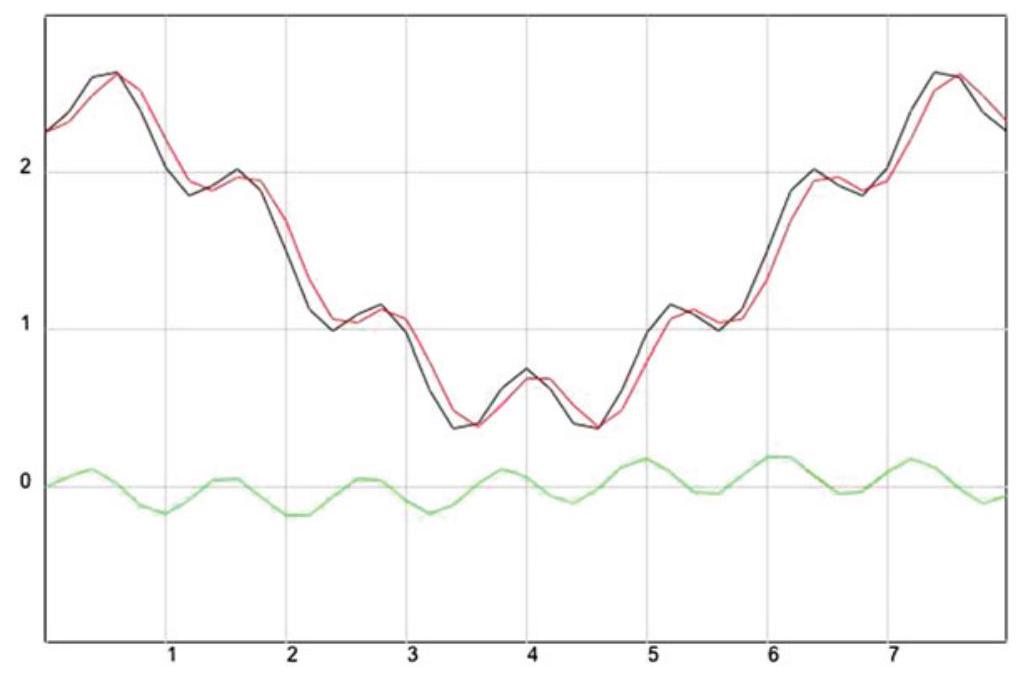
\[ \begin{array}{rlll} \frac{1}{2}\left(x_{1}+x_{2}\right)=y_{2} & \frac{1}{2}\left(x_{3}+x_{4}\right)=y_{4} & \frac{1}{2}\left(x_{5}+x_{6}\right)=y_{6} \\ \frac{1}{2}\left(-x_{1}+x_{2}\right)=z_{2} & \frac{1}{2}\left(-x_{3}+x_{4}\right)=z_{4} & \frac{1}{2}\left(-x_{5}+x_{6}\right)=z_{6} \end{array} \]
. . .
\[ A_{6} \mathbf{x} \equiv \frac{1}{2}\left[\begin{array}{rrrrrr} 1 & 1 & 0 & 0 & 0 & 0 \\ 0 & 0 & 1 & 1 & 0 & 0 \\ 0 & 0 & 0 & 0 & 1 & 1 \\ -1 & 1 & 0 & 0 & 0 & 0 \\ 0 & 0 & -1 & 1 & 0 & 0 \\ 0 & 0 & 0 & 0 & -1 & 1 \end{array}\right]\left[\begin{array}{l} x_{1} \\ x_{2} \\ x_{3} \\ x_{4} \\ x_{5} \\ x_{6} \end{array}\right]=\left[\begin{array}{l} y_{2} \\ y_{4} \\ y_{6} \\ z_{2} \\ z_{4} \\ z_{6} \end{array}\right] \]
Almost orthogonal
\[ \begin{aligned} A_{6} A_{6}^{T} &=\frac{1}{4}\left[\begin{array}{rrrrrr} 1 & 1 & 0 & 0 & 0 & 0 \\ 0 & 0 & 1 & 1 & 0 & 0 \\ 0 & 0 & 0 & 0 & 1 & 1 \\ -1 & 1 & 0 & 0 & 0 & 0 \\ 0 & 0 & -1 & 1 & 0 & 0 \\ 0 & 0 & 0 & 0 & -1 & 1 \end{array}\right]\left[\begin{array}{cccccc} 1 & 0 & 0 & -1 & 0 & 0 \\ 1 & 0 & 0 & 1 & 0 & 0 \\ 0 & 1 & 0 & 0 & -1 & 0 \\ 0 & 1 & 0 & 0 & 1 & 0 \\ 0 & 0 & 1 & 0 & 0 & -1 \\ 0 & 0 & 1 & 0 & 0 & 1 \end{array}\right] \\[10pt] &=\frac{1}{2}\left[\begin{array}{llllll} 1 & 0 & 0 & 0 & 0 & 0 \\ 0 & 1 & 0 & 0 & 0 & 0 \\ 0 & 0 & 1 & 0 & 0 & 0 \\ 0 & 0 & 0 & 1 & 0 & 0 \\ 0 & 0 & 0 & 0 & 1 & 0 \\ 0 & 0 & 0 & 0 & 0 & 1 \end{array}\right]=\frac{1}{2} I_{6} \end{aligned} \]
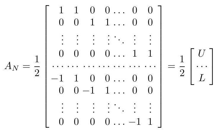
In general,
\(A_{N} A_{N}^{T}=\frac{1}{2} I_{N}\)
. . .
These matrices are nearly orthogonal.
Haar Wavelet Transform Matrix
Can make them orthogonal by dividing by \(\sqrt{2}\):
\[ y_{k}=\frac{\sqrt{2}}{2}\left(x_{k}+x_{k-1}\right), \quad k \in \mathbb{Z} \]
and
\[ z_{k}=\frac{\sqrt{2}}{2}\left(x_{k}-x_{k-1}\right), \quad k \in \mathbb{Z} \]
. . .
\[ W_{N}=\frac{\sqrt{2}}{2}\left[\begin{array}{ccccccc} 1 & 1 & 0 & 0 & \ldots & 0 & 0 \\ 0 & 0 & 1 & 1 & \ldots & 0 & 0 \\ \vdots & \vdots & \vdots & \vdots & \ddots & \vdots & \vdots \\ 0 & 0 & 0 & 0 & \ldots & 1 & 1 \\ \ldots & \ldots & \ldots & \ldots & \ldots & \ldots \\ -1 & 1 & 0 & 0 & \ldots & 0 & 0 \\ 0 & 0 & -1 & 1 & \ldots & 0 & 0 \\ \vdots & \vdots & \vdots & \vdots & \ddots & \vdots & \vdots \\ 0 & 0 & 0 & 0 & \ldots & -1 & 1 \end{array}\right]=\frac{\sqrt{2}}{2}\left[\begin{array}{c} U \\ \ldots \\ L \end{array}\right] \]
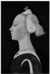
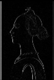
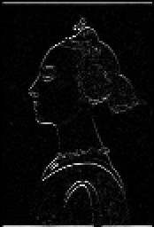
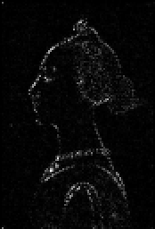
Moving to 2D
For a 2D image represented pixel-by-pixel in the matrix \(\mathbf{A}\), we can apply the 1D transform to each row and then to each column: \(W_{m} A W_{n}^{T}\)
. . .
Result ends up in block form:
\[ W_{m} A W_{n}^{T}=2\left[\begin{array}{ll} B & V \\ H & D \end{array}\right] \]
. . .
![]()
. . .
\(B\) represents the blurred image of \(A\), while \(V\), \(H\) and \(D\) represent edges along vertical, horizontal and diagonal directions.
. . .
Reconstructing the original
What we have: The four blocks from the forward transform — the blur \(B\) (top-left), vertical edges \(V\) (top-right), horizontal edges \(H\) (bottom-left), and diagonal edges \(D\) (bottom-right). Each block is half the height and half the width of the original image.
What we want: The original image \(A\) (same size as before the transform).
1. Put the four blocks back into one matrix T in the same layout they came from:
   - Top-left of T    = 2*B    (blur)
   - Top-right of T  = 2*V    (vertical edges)
   - Bottom-left of T = 2*H    (horizontal edges)
   - Bottom-right of T = 2*D   (diagonal edges)
   The factor 2 matches the forward formula W_m A W_n^T = 2[B V; H D].

2. Undo the transform. The forward step was "apply W to rows, then W to columns."
   The inverse is: apply W^T to rows of T, then W^T to columns.
   So:  A = W_m^T * T * W_n
   (Same Haar matrices W_m, W_n as before; orthogonality gives W^T = W^{-1}.)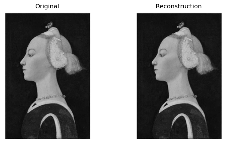
. . .
Skills
- Describe the 1D Haar transform: average and difference filters; recovery of the original signal.
- Recognize that the Haar matrices satisfy \(A_N A_N^T = \frac{1}{2}I_N\) (nearly orthogonal); scaling by \(\sqrt{2}\) gives an orthogonal \(W_N\).
- For 2D images, apply the 1D transform by rows then columns: \(W_m A W_n^T\); interpret the blocks \(B\), \(V\), \(H\), \(D\).