Ch5 Lecture 1

Outline for today

• Eigenvalues and Eigenvectors
• Similarity and Diagonalization
• Application to Discrete Dynamical Systems

Eigenvalues and Eigenvectors

Eigenvalues and Eigenvectors

An eigenvector of A is a nonzero vector \mathbf{x} in \mathbb{R}^{n} (or \mathbb{C}^{n}) such that for some scalar \lambda, we have

A \mathbf{x}=\lambda \mathbf{x}

Why do we care? One reason: matrix multiplication can become scalar multiplication:

\begin{aligned} A \mathbf{x} & =\lambda \mathbf{x} \\ A^{2} \mathbf{x} & =A(A \mathbf{x})=A \lambda \mathbf{x}=\lambda A \mathbf{x}=\lambda^{2} \mathbf{x} \\ & \vdots \\ A^{k} \mathbf{x} & =A\left(A^{k-1} \mathbf{x}\right)=\cdots=\lambda^{k} \mathbf{x} . \end{aligned}

Will see how to use these ideas to understand dynamics even for vectors that aren’t eigenvectors.

Finding Eigenvalues and Eigenvectors

\lambda is an eigenvalue of A if A \mathbf{x}=\lambda \mathbf{x}\left(=\lambda I \mathbf{x}\right)

\mathbf{0}=\lambda I \mathbf{x}-A \mathbf{x}=(\lambda I-A) \mathbf{x}

pause

Remember a system of equations A \mathbf{x}=0 has a non-trivial solution if and only if A is singular, or in other words \operatorname{det}(A)=0.

So, \lambda is an eigenvalue of A \iff \operatorname{det}(\lambda I-A)=0.

If A is a square n \times n matrix, the equation \operatorname{det}(\lambda I-A)=0 is called the characteristic equation of A, and the n th-degree monic polynomial p(\lambda)=\operatorname{det}(\lambda I-A) is called the characteristic polynomial of A.

Eigenspaces and Eigensystems

The eigenspace corresponding to eigenvalue \lambda is the subspace \mathcal{N}(\lambda I-A) of \mathbb{R}^{n} (or \left.\mathbb{C}^{n}\right).

We write \mathcal{E}_{\lambda}(A)=\mathcal{N}(\lambda I-A).

Note: \mathbf{0} is in every eigenspace, but it is not an eigenvector.

The eigensystem of the matrix A is a list of all the eigenvalues of A and, for each eigenvalue \lambda, a complete description of its eigenspace – usually a basis.

Eigensystem Algorithm:

Given n \times n matrix A, to find an eigensystem for A :

1. Find the eigenvalues of A.

2. For each scalar \lambda in (1), use the null space algorithm to find a basis of the eigenspace \mathcal{N}(\lambda I-A).

A reminder: the Null Space algorithm

Given an m \times n matrix A.

1. Compute the reduced row echelon form R of A.

2. Use R to find the general solution to the homogeneous system A \mathbf{x}=0.

3. Write the general solution \mathbf{x}=\left(x_{1}, x_{2}, \ldots, x_{n}\right) to the homogeneous system in the form

\mathbf{x}=x_{i_{1}} \mathbf{w}_{1}+x_{i_{2}} \mathbf{w}_{2}+\cdots+x_{i_{n-r}} \mathbf{w}_{n-r}

where x_{i_{1}}, x_{i_{2}}, \ldots, x_{i_{n-r}} are the free variables.

4. List the vectors \mathbf{w}_{1}, \mathbf{w}_{2}, \ldots, \mathbf{w}_{n-r}. These form a basis of \mathcal{N}(A).

Example of the Null Space algorithm

Find a basis for the null space of the matrix A=\left[\begin{array}{llll} 1 & 0 & 1 & 2 \\ 1 & 2 & 0 & 1 \\ 3 & 2 & 2 & 5 \\ 3 & 4 & 1 & 4 \end{array}\right]

The reduced row echelon form of A is

R=\left[\begin{array}{rrrr} 1 & 0 & 1 & 2 \\ 0 & 1 & -1 / 2 & -1 / 2 \\ 0 & 0 & 0 & 0 \\ 0 & 0 & 0 & 0 \end{array}\right]

The variables x_{3} and x_{4} are free, while x_{1} and x_{2} are bound.

Hence, the general solution of A \mathbf{x}=0 can be written as

\begin{aligned} x_{1} & =-x_{3}-2 x_{4}, \\ x_{2} & =\frac{1}{2} x_{3}+\frac{1}{2} x_{4}, \\ x_{3} & =x_{3}, \\ x_{4} & =x_{4}, \end{aligned}

\left[\begin{array}{l} x_{1} \\ x_{2} \\ x_{3} \\ x_{4} \end{array}\right]=x_{3}\left[\begin{array}{r} -1 \\ 1 / 2 \\ 1 \\ 0 \end{array}\right]+x_{4}\left[\begin{array}{r} -2 \\ 1 / 2 \\ 0 \\ 1 \end{array}\right] .

which becomes, in vector notation,

\left[\begin{array}{l} x_{1} \\ x_{2} \\ x_{3} \\ x_{4} \end{array}\right]=x_{3}\left[\begin{array}{r} -1 \\ 1 / 2 \\ 1 \\ 0 \end{array}\right]+x_{4}\left[\begin{array}{r} -2 \\ 1 / 2 \\ 0 \\ 1 \end{array}\right] .

:::

Example

Find an eigensystem for the matrix A=\left[\begin{array}{ll}7 & 4 \\ 3 & 6\end{array}\right]

\begin{aligned} 0 & =\operatorname{det}(\lambda I-A)=\operatorname{det}\left[\begin{array}{rr} \lambda-7 & -4 \\ -3 & \lambda-6 \end{array}\right] \\ & =(\lambda-7)(\lambda-6)-(-3)(-4) \\ & =\lambda^{2}-13 \lambda+42-12 \\ & =\lambda^{2}-13 \lambda+30 \\ & =(\lambda-3)(\lambda-10) . \end{aligned}

Eigenvalues are \lambda=3 and \lambda=10.

For \lambda=3, we have

A-3 I=\left[\begin{array}{rr} 7-3 & 4 \\ 3 & 3-3 \end{array}\right] = {\left[\begin{array}{ll} 4 & 4 \\ 3 & 3 \end{array}\right] \xrightarrow[E_{21}(-3 / 4)]{E_{1}(1 / 4)}\left[\begin{array}{ll} 1 & 1 \\ 0 & 0 \end{array}\right]}

So x_{2} is free and x_{1} is bound, x_{1}=-x_{2},so

\left[\begin{array}{l} x_{1} \\ x_{2} \end{array}\right]=\left[\begin{array}{c} -x_{2} \\ x_{2} \end{array}\right]=x_{2}\left[\begin{array}{r} -1 \\ 1 \end{array}\right]

so the eigenspace is spanned by \left[\begin{array}{l}1 \\ -1\end{array}\right].

Thus, a basis of \mathcal{E}_{3}(A) is \{(-1,1)\}.

Similarly, for \lambda=10, the basis of \mathcal{E}_{10}(A) is \{(4 / 3,1)\}

Two examples with repeated eigenvalues

What happens when an eigenvalue is repeated?

Example: find the eigenspace for eigenvalue \lambda=2 of these two matrices:

\text { (a) }\left[\begin{array}{rrr} 2 & 1 & 2 \\ 0 & 1 & -2 \\ 0 & 0 & 2 \end{array}\right] \quad \text { (b) }\left[\begin{array}{lll} 2 & 1 & 1 \\ 0 & 1 & 1 \\ 0 & 0 & 2 \end{array}\right]

Both matrices have eigenvalues \lambda=1,2,2, but their eigenspaces for \lambda=2 are different:

After row reducing the first matrix, we get

\left[\begin{array}{rrr} 0 & 1 & 2 \\ 0 & -1 & -2 \\ 0 & 0 & 0 \end{array}\right] \xrightarrow[E_{21}(1)]{\longrightarrow}\left[\begin{array}{lll} 0 & 1 & 2 \\ 0 & 0 & 0 \\ 0 & 0 & 0 \end{array}\right]

\left[\begin{array}{l} x_{1} \\ x_{2} \\ x_{3} \end{array}\right]=\left[\begin{array}{c} x_{1} \\ -2 x_{3} \\ x_{3} \end{array}\right]=x_{1}\left[\begin{array}{l} 1 \\ 0 \\ 0 \end{array}\right]+x_{3}\left[\begin{array}{r} 0 \\ -2 \\ 1 \end{array}\right] .

A basis for \mathcal{E}_{2}(A) is \{(1,0,0),(0,-2,1)\}.

Dimension of \mathcal{E}_{2}(A)=2.

\text { (a) }\left[\begin{array}{rrr} 2 & 1 & 2 \\ 0 & 1 & -2 \\ 0 & 0 & 2 \end{array}\right] \quad \text { (b) }\left[\begin{array}{lll} 2 & 1 & 1 \\ 0 & 1 & 1 \\ 0 & 0 & 2 \end{array}\right]

For the second matrix, we have \left[\begin{array}{rrr} 0 & 1 & 1 \\ 0 & -1 & 1 \\ 0 & 0 & 0 \end{array}\right] \xrightarrow[E_{21}(1)]{\longrightarrow}\left[\begin{array}{lll} 0 & 1 & 1 \\ 0 & 0 & 2 \\ 0 & 0 & 0 \end{array}\right] \xrightarrow{E_{2}(1 / 2)}\left[\begin{array}{lll} 0 & 1 & 0 \\ 0 & 0 & 1 \\ 0 & 0 & 0 \end{array}\right]

Only free variable is x_{1}, so

\left[\begin{array}{l} x_{1} \\ x_{2} \\ x_{3} \end{array}\right]=\left[\begin{array}{c} x_{1} \\ 0 \\ 0 \end{array}\right]=x_{1}\left[\begin{array}{l} 1 \\ 0 \\ 0 \end{array}\right]

A basis for \mathcal{E}_{2}(A) is \{(1,0,0)\}. Dimension of \mathcal{E}_{2}(A)=1.

Eigenvalue Multiplicity

The algebraic multiplicity of \lambda is the multiplicity of \lambda as a root of the characteristic equation. The geometric multiplicity of \lambda is the dimension of the space \mathcal{E}_{\lambda}(A)=\mathcal{N}(\lambda I-A).

The eigenvalue \lambda of A is said to be simple if its algebraic multiplicity is 1 , that is, the number of times it occurs as a root of the characteristic equation is 1 . Otherwise, the eigenvalue is said to be repeated.

For an n \times n matrix A, the sum of the algebraic multiplicities of all the eigenvalues of A is n.

(In other words, there are n eigenvalues, counting algebraic multiplicities and complex numbers).

The geometric multiplicity of an eigenvalue is always less than or equal to its algebraic multiplicity.

Defective Matrices

A matrix is defective if one of its eigenvalues has geometric multiplicity less than its algebraic multiplicity.

This means that the sum of the geometric multiplicities of all the eigenvalues is less than n.

Similarity and Diagonalization

Functions of Diagonal Matrices

It’s easy to find functions of matrices if the matrix is diagonal.

D = \operatorname{diag}\left\{\lambda_{1}, \lambda_{2}, \lambda_{3}\right\}=\left[\begin{array}{ccc} \lambda_{1} & 0 & 0 \\ 0 & \lambda_{2} & 0 \\ 0 & 0 & \lambda_{3} \end{array}\right]

D^{k}=\operatorname{diag}\left\{\lambda_{1}^{k}, \lambda_{2}^{k}, \ldots, \lambda_{n}^{k}\right\}

f(D)=\operatorname{diag}\left\{f\left(\lambda_{1}\right), f\left(\lambda_{2}\right), \ldots, f\left(\lambda_{n}\right)\right\}

Similar Matrices

A matrix A is said to be similar to matrix B if there exists an invertible matrix P such that

P^{-1} A P=B .

P is called a similarity transformation matrix.

If A is similar to M, say P^{-1} A P=M. Then:

1. For every polynomial q(x), q(M)=P^{-1} q(A) P .

2. The matrices A and M have the same eigenvalues.

So in particular,

\begin{equation*} A^{k}=P D^{k} P^{-1} \end{equation*}

Diagonalization

Suppose we have a 3 \times 3 matrix A

Suppose we then find three linearly independent eigenvectors \mathbf{v}_{1}, \mathbf{v}_{2}, \mathbf{v}_{3}

A \mathbf{v}_{1}=\lambda_{1} \mathbf{v}_{1}, A \mathbf{v}_{2}=\lambda_{2} \mathbf{v}_{2}

A \mathbf{v}_{1}=\lambda_{1} \mathbf{v}_{1}, A \mathbf{v}_{2}=\lambda_{2} \mathbf{v}_{2} etc

Put this together: A\left[\mathbf{v}_{1}, \mathbf{v}_{2}, \mathbf{v}_{3}\right]=\left[\mathbf{v}_{1}, \mathbf{v}_{2}, \mathbf{v}_{3}\right]\left[\begin{array}{ccc} \lambda_{1} & 0 & 0 \\ 0 & \lambda_{2} & 0 \\ 0 & 0 & \lambda_{3} \end{array}\right]=\left[\mathbf{v}_{1}, \mathbf{v}_{2}, \mathbf{v}_{3}\right] \operatorname{diag}\left\{\lambda_{1}, \lambda_{2}, \lambda_{3}\right\}

Now define P=\left[\mathbf{v}_{1}, \mathbf{v}_{2}, \mathbf{v}_{3}\right] and D=\operatorname{diag}\left\{\lambda_{1}, \lambda_{2}, \lambda_{3}\right\}

Multiply on the right by P^{-1} (can do because columns of P are linearly independent, so it’s invertible):

A P=P D\Rightarrow P^{-1} D P=A

To diagonalize an n \times n matrix A, we just need to find n independent eigenvectors and put them into the columns of a matrix P. Then P^{-1} A P=D

Example

Find f(A) for A=\left[\begin{array}{rrr} 2 & 1 & 2 \\0 & 1 & -2 \\0 & 0 & 2\end{array}\right] with f(x)=\sin \left(\frac{\pi}{2} x\right)

From before, the basis vectors for the eigenspace of \lambda=2 are \{(1,0,0),(0,-2,1)\}

The basis for the eigenspace of \lambda=1 is \{(-1,1,0)\}

P=\left[\mathbf{v}_{1}, \mathbf{v}_{2}, \mathbf{v}_{3}\right]=\left[\begin{array}{rrr} 1 & 0 & -1 \\ 0 & -2 & 1 \\ 0 & 1 & 0 \end{array}\right] .

P^{-1}=\left[\begin{array}{lll} 1 & 1 & 2 \\ 0 & 0 & 1 \\ 0 & 1 & 2 \end{array}\right]

P^{-1} A P=\left[\begin{array}{lll} 2 & 0 & 0 \\ 0 & 2 & 0 \\ 0 & 0 & 1 \end{array}\right]=D

\begin{aligned} \sin \left(\frac{\pi}{2} A\right)&=P^{-1} \sin \left(\frac{\pi}{2} D\right) P \\[20pt] &= \left[\begin{array}{rrr}1 & 0 & -1 \\ 0 & -2 & 1 \\ 0 & 1 & 0\end{array}\right]\left[\begin{array}{ccc}\sin \left(2 \frac{\pi}{2}\right) & 0 & 0 \\ 0 & \sin \left(2 \frac{\pi}{2}\right) & 0 \\ 0 & 0 & \sin \left(1 \frac{\pi}{2}\right)\end{array}\right]\left[\begin{array}{lll}1 & 1 & 2 \\ 0 & 0 & 1 \\ 0 & 1 & 2\end{array}\right]\\[10pt] &=\left[\begin{array}{ccc}0 & -1 & -2 \\ 0 & 1 & 2 \\ 0 & 0 & 0\end{array}\right] \end{aligned}

When are matrices diagonalizable?

The n \times n matrix A is diagonalizable if and only if there exists a linearly independent set of eigenvectors \mathbf{v}_{1}, \mathbf{v}_{2}, \ldots, \mathbf{v}_{n} of A \dots in which case P=\left[\mathbf{v}_{1}, \mathbf{v}_{2}, \ldots, \mathbf{v}_{n}\right] is a diagonalizing matrix for A.

If the n \times n matrix A has n distinct eigenvalues, then A is diagonalizable.

Caution: Just because the n \times n matrix A has fewer than n distinct eigenvalues, you may not conclude that it is not diagonalizable.

Application to Discrete Dynamical Systems

Diagonalizable Transition Matrices

Suppose you have the discrete dynamical system \mathbf{x}^{(k+1)}=A \mathbf{x}^{(k)}

Assume A is diagonalizable, then we can write complete, linearly independent eigenvectors \mathbf{v}_{1}, \mathbf{v}_{2}, \ldots, \mathbf{v}_{n}, with eigenvalues \lambda_{1}, \lambda_{2}, \ldots, \lambda_{n}.

Suppose the eigenvalues are ordered, so that |\lambda_{1}| \geq|\lambda_{2}| \geq \cdots \geq|\lambda_{n}|.

Then the eigenvectors form a basis of \mathbb{R}^{n} (or \mathbb{C}^{n}), so we can express our initial state as a linear combination of the eigenvectors: \begin{equation*} \mathbf{x}^{(0)}=c_{1} \mathbf{v}_{1}+c_{2} \mathbf{v}_{2}+\cdots+c_{n} \mathbf{v}_{n} \end{equation*}

Now we know the effect of multiplying by A:

\begin{aligned} A \mathbf{x}^{(0)} & =A\left(c_{1} \mathbf{v}_{1}+c_{2} \mathbf{v}_{2}+\cdots+c_{n} \mathbf{v}_{n}\right) \\ & =c_{1}\left(A \mathbf{v}_{1}\right)+c_{2}\left(A \mathbf{v}_{2}\right)+\cdots+c_{n}\left(A \mathbf{v}_{n}\right) \\ & =c_{1} \lambda_{1} \mathbf{v}_{1}+c_{2} \lambda_{2} \mathbf{v}_{2}+\cdots+c_{n} \lambda_{n} \mathbf{v}_{n} \end{aligned}

Can do it repeatedly: \begin{equation*} \mathbf{x}^{(k)}=c_{1} \lambda_{1}^{k} \mathbf{v}_{1}+c_{2} \lambda_{2}^{k} \mathbf{v}_{2}+\cdots+c_{n} \lambda_{n}^{k} \mathbf{v}_{n} \end{equation*}

Spectral Radius and Dominant Eigenvalue

\begin{equation*} \mathbf{x}^{(k)}=c_{1} \lambda_{1}^{k} \mathbf{v}_{1}+c_{2} \lambda_{2}^{k} \mathbf{v}_{2}+\cdots+c_{n} \lambda_{n}^{k} \mathbf{v}_{n} \end{equation*}

What will happen when \lambda_{1} is greater than 1? Equal to one? Less than one? What about the others?

The spectral radius \rho(A) of a matrix A with eigenvalues \lambda_{1}, \lambda_{2}, \ldots, \lambda_{n} is

\rho(A)=\max \left\{\left|\lambda_{1}\right|,\left|\lambda_{2}\right|, \ldots,\left|\lambda_{n}\right|\right\} .

If \left|\lambda_{k}\right|=\rho(A) and \lambda_{k} is the only eigenvalue with this property, then \lambda_{k} is the dominant eigenvalue of A.

Implications of the Spectral Radius

For n \times n transition matrix A, initial state vector \mathbf{x}^{(0)}:

1. If \rho(A)<1, then \lim _{k \rightarrow \infty} A^{k} \mathbf{x}^{(0)}=\mathbf{0}.

2. If \rho(A)=1, then the sequence of norms \left\{\left\|\mathbf{x}^{(k)}\right\|\right\}_{k=0}^{\infty} is bounded.

3. If \rho(A)=1 and \lambda=1 is the dominant eigenvalue of A, then \lim _{k \rightarrow \infty} \mathbf{x}^{(k)} is an element of \mathcal{E}_{1}(A) – either an eigenvector or \mathbf{0}.

4. If \rho(A)>1, then for some choices of \mathbf{x}^{(0)} we have \lim _{k \rightarrow \infty}\|\mathbf{x}\|=\infty

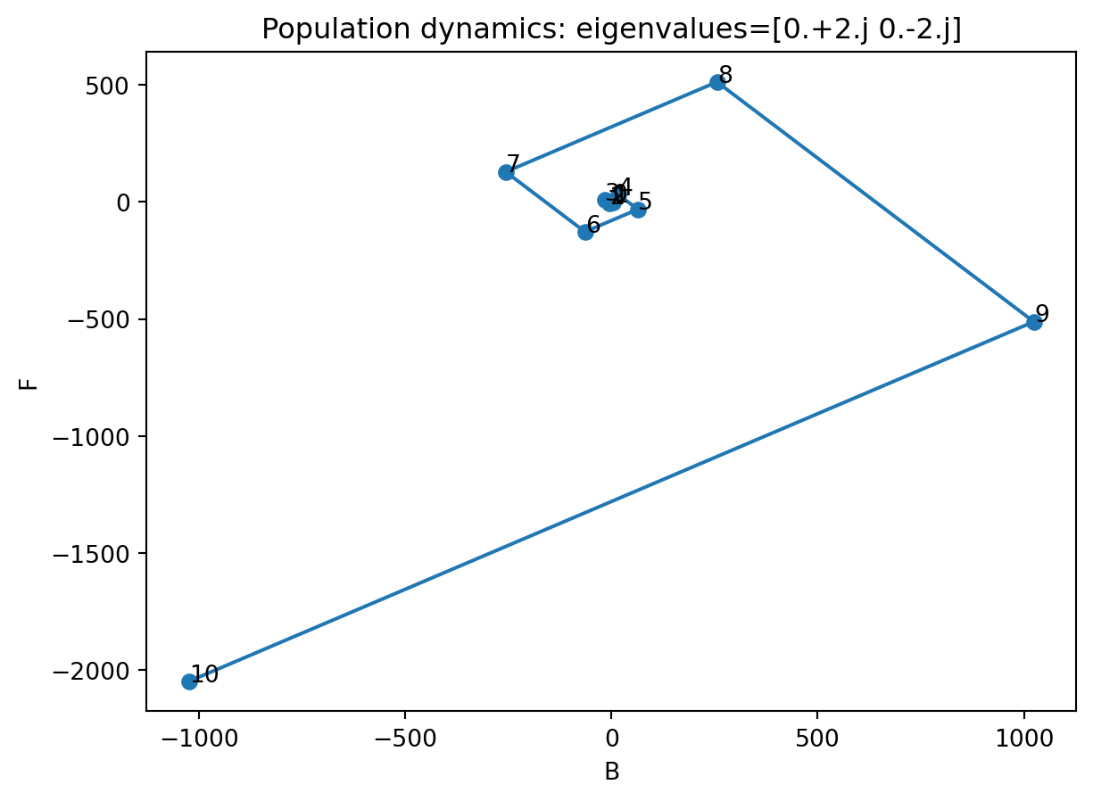
Example

You have too many frogs.

There is a species of bird that eats frogs. (Yay!) Can these help you with your frog problem?

Let F_{k} and B_{k} be the number of frogs and birds at year k.

\begin{aligned} B_{k+1} & =0.6 B_{k}+0.4 F_{k}, \\ F_{k+1} & =-r B_{k}+1.4 F_{k}, \end{aligned}

where r is the rate at which the birds eat the frogs. (Suppose it’s around 0.35).

There are some issues with this model. You can end up with negative frogs. And you can have birds appear from nowhere. But let’s ignore that for now.

Is it a good idea to introduce these birds?

Let the population vector in the k th year be \mathbf{x}^{(k)}=\left(B_{k}, F_{k}\right)

\left[\begin{array}{l} B_{k+1} \\ F_{k+1} \end{array}\right]=\left[\begin{array}{rr} 0.6 & 0.4 \\ -0.35 & 1.4 \end{array}\right]\left[\begin{array}{l} B_{k} \\ F_{k} \end{array}\right]

Find eigenvalues and eigenvectors of the transition matrix.

import numpy as np
A = np.array([[0.6, 0.4], [-0.35, 1.4]])
eigvals, eigvecs = np.linalg.eig(A)
eigvals_sorted = np.sort(eigvals)[::-1]
eigvecs_sorted = eigvecs[:, np.argsort(eigvals)[::-1]]
print('Eigenvalues: ' + str(eigvals_sorted))
print('Eigenvectors: '+ str(eigvecs_sorted))

Eigenvalues: [1.14142136 0.85857864]
Eigenvectors: [[-0.59421716 -0.83980458]
 [-0.80430465 -0.54288882]]

Check: use Sympy to diagonalize the matrix.

D : Matrix([[0.858578643762691, 0], [0, 1.14142135623731]])
P : Matrix([[0.839804577036026, 0.635068381284203], [0.542888821389189, 0.859598960745815]])

\displaystyle \left[\begin{matrix}0.6 & 0.4\\-0.35 & 1.4\end{matrix}\right]

What this means is that the component of the initial vector which is in the direction of the eigenvector corresponding to the dominant eigenvalue will grow exponentially, while the other component will decay.

Unless we start only with a vector that’s proportional to the second eigenvector, the frog population will explode.

x0 = np.array([100, 10000]) 

def print_iterations(x0, A, n1=10, n2=1):
  x = x0
  for i in range(n1):
    for j in range(n2):
      x = A @ x
    print(x)


print_iterations(x0, A)

[ 4060. 13965.]
[ 8022. 18130.]
[12065.2 22574.3]
[16268.84 27381.2 ]
[20713.784 32639.586]
[25484.1048 38445.596 ]
[30668.70128 44904.39772]
[36362.979856 52132.11136 ]
[42670.6324576 60257.9129544]
[49705.54465632 69426.356776  ]

Different starting points…

x0 = eigvecs_sorted[0]*-1000
print_iterations(x0, A)

[692.45212576 967.75040247]
[ 802.57143644 1112.49231944]
[ 926.53978964 1276.58924446]
[1066.55957157 1462.93601587]
[1225.11014929 1674.81457217]
[1404.99191844 1915.95184879]
[1609.37589058 2190.58541685]
[1841.85970109 2503.53802188]
[2106.5310294  2860.30233525]
[2408.03955174 3267.13740907]

What if we start with the second eigenvector?

x0 = eigvecs_sorted[1]*-1000
print_iterations(x0, A)

[699.73831812 478.5377227 ]
[611.25807995 425.04440043]
[536.77260814 381.12183262]
[474.51229793 345.70015282]
[422.98743989 317.90090967]
[380.9528278  297.01566957]
[347.37796451 282.48844767]
[321.42215777 273.90153916]
[302.41391033 270.96439961]
[289.83410604 273.50529084]

Looks good so far, doesn’t blow up. But if we continue (only printing results every 10 years now):

x0 = eigvecs_sorted[1]*-1000
print_iterations(x0, A,n1 = 10, n2 = 10)

[289.83410604 273.50529084]
[493.86429346 642.61221892]
[1724.50444871 2328.57998379]
[6445.12974686 8722.60198143]
[24186.97763221 32738.09888286]
[ 90789.4036837  122888.24713326]
[340796.1924577  461285.82916599]
[1279247.72362158 1731530.09096614]
[4801916.36748821 6499650.17996028]
[18024969.23527191 24397758.22361141]

Even the roundoff errors are starting to make the frog population explode

What about complex eigenvalues?

Let’s repeat the above for a different matrix:

\left[\begin{array}{ll} 0 & 2 \\ -2 & 0 \end{array}\right]

A = np.array([[0, 2], [-2, 0]])
eigvals, eigvecs = np.linalg.eig(A)
eigvals_sorted = np.sort(eigvals)[::-1]
eigvecs_sorted = eigvecs[:, np.argsort(eigvals)[::-1]]
print('Eigenvalues: ' + str(eigvals_sorted))
print('Eigenvectors: '+ str(eigvecs_sorted))
print_iterations(np.array([1,2]), A,n1 = 10, n2 = 1)

Eigenvalues: [0.+2.j 0.-2.j]
Eigenvectors: [[0.        -0.70710678j 0.        +0.70710678j]
 [0.70710678+0.j         0.70710678-0.j        ]]
[ 4 -2]
[-4 -8]
[-16   8]
[16 32]
[ 64 -32]
[ -64 -128]
[-256  128]
[256 512]
[1024 -512]
[-1024 -2048]

Let’s plot that…

import matplotlib.pyplot as plt

def plot_iterations(x0, A, n1=10, n2=1):
  plt.clf()
  x = x0
  x_vals = [x]
  for i in range(n1):
    for j in range(n2):
      x = A @ x
    x_vals.append(x)
  x_vals = np.array(x_vals)
  plt.plot(x_vals[:,0], x_vals[:,1], 'o-',)
  for i, txt in enumerate(range(len(x_vals))):
    plt.annotate(txt, (x_vals[i,0]+1, x_vals[i,1]+1))
  #plt.plot(x_vals[:,0], x_vals[:,1], 'o-')
  plt.xlabel('B')
  plt.ylabel('F')
  plt.title('Population dynamics: eigenvalues='+str(np.linalg.eig(A)[0]))
  plt.show()

Your turn

Another example

Fibonacci Statue

Fibonacci sequence: 0, 1, 1, 2, 3, 5, 8, 13, 21, …

F_{0}=0 and F_{1}=1. For n \geq 2, the n-th Fibonacci number is

F_{n}=F_{n-1}+F_{n-2}

What is the n-th Fibonacci number? What is F_{100}?

(Treatment from here)

Get this into matrix form.

Let \bar{x}_{k}=\left[\begin{array}{c} F_{k} \\ F_{k+1} \end{array}\right]

Then

\bar{x}_{k+1}=\left[\begin{array}{c} F_{k+1} \\ F_{k+2} \end{array}\right]=\left[\begin{array}{c} F_{k+1} \\ F_{k}+F_{k+1} \end{array}\right]=\left[\begin{array}{ll} 0 & 1 \\ 1 & 1 \end{array}\right]\left[\begin{array}{c} F_{k} \\ F_{k+1} \end{array}\right]=\left[\begin{array}{ll} 0 & 1 \\ 1 & 1 \end{array}\right] \bar{x}_{k}

for \bar{x}_{0}=\left[\begin{array}{l}0 \\1\end{array}\right]

To understand the dynamics, we need to diagonalize the matrix.

\begin{aligned} \operatorname{det}(A-\lambda I) & =0 \\ \operatorname{det}\left[\begin{array}{cc} -\lambda & 1 \\ 1 & 1-\lambda \end{array}\right] & =0 \\ \lambda^{2}-\lambda-1 & =0 \\ \lambda & =\frac{1 \pm \sqrt{5}}{2} \end{aligned}

Eigenvalues (call them phi and psi): \begin{aligned} & \varphi=\frac{1+\sqrt{5}}{2} \approx 1.618 \\ & \psi=\frac{1-\sqrt{5}}{2} \approx-0.618 \end{aligned}

Eigenvectors:

\bar{v}_{\varphi}=\left[\begin{array}{l} 1 \\ \varphi \end{array}\right] \quad \text { and } \quad \bar{v}_{\psi}=\left[\begin{array}{l} 1 \\ \psi \end{array}\right]

A=P D P^{-1}=\left[\begin{array}{ll} 1 & 1 \\ \varphi & \psi \end{array}\right]\left[\begin{array}{ll} \varphi & 0 \\ 0 & \psi \end{array}\right] \frac{1}{\sqrt{5}}\left[\begin{array}{cc} -\psi & 1 \\ \varphi & -1 \end{array}\right]

\begin{aligned} & A^{k}=P D^{k} P^{-1} \\ & =\left[\begin{array}{cc} 1 & 1 \\ \varphi & \psi \end{array}\right]\left[\begin{array}{cc} \varphi^{k} & 0 \\ 0 & \psi^{k} \end{array}\right] \frac{1}{\sqrt{5}}\left[\begin{array}{cc} -\psi & 1 \\ \varphi & -1 \end{array}\right] \\ & =\left[\begin{array}{cc} \varphi^{k} & \psi^{k} \\ \varphi^{k+1} & \psi^{k+1} \end{array}\right] \frac{1}{\sqrt{5}}\left[\begin{array}{cc} -\psi & 1 \\ \varphi & -1 \end{array}\right] \\ & =\frac{1}{\sqrt{5}}\left[\begin{array}{cc} -\psi \varphi^{k}+\varphi \psi^{k} & \varphi^{k}-\psi^{k} \\ -\psi \varphi^{k+1}+\varphi \psi^{k+1} & \varphi^{k+1}-\psi^{k+1} \end{array}\right] \end{aligned}

Finally,

\left[\begin{array}{c} F_{k} \\ F_{k+1} \end{array}\right]=A^{k} \bar{x}_{0}=\frac{1}{\sqrt{5}}\left[\begin{array}{cc} -\psi \varphi^{k}+\varphi \psi^{k} & \varphi^{k}-\psi^{k} \\ -\psi \varphi^{k+1}+\varphi \psi^{k+1} & \varphi^{k+1}-\psi^{k+1} \end{array}\right]\left[\begin{array}{l} 0 \\ 1 \end{array}\right]=\frac{1}{\sqrt{5}}\left[\begin{array}{c} \varphi^{k}-\psi^{k} \\ \varphi^{k+1}-\psi^{k+1} \end{array}\right]

and so

F_{k}=\frac{1}{\sqrt{5}}\left(\varphi^{k}-\psi^{k}\right)=\frac{1}{\sqrt{5}}\left(\left(\frac{1+\sqrt{5}}{2}\right)^{k}+\left(\frac{1-\sqrt{5}}{2}\right)^{k}\right)

But for large k, \psi^{k} is very small, so

F_{k} \approx \frac{\varphi^{k}}{\sqrt{5}}

\lim _{k \rightarrow \infty} \frac{F_{k+1}}{F_{k}}=\varphi

This is the golden ratio!

Golden Ratio spiral

Go back to some of the previous examples we’ve used, or that you’ve used in your projects. Work in pairs to find the eigenvalues and eigenvectors of the transition matrix. What do the eigenvalues tell you about the dynamics of the system?