Ch 5 Lecture 3

Outline for today

• Intuition about SVD
• Uses of SVD
• Matrices as data

Intuition about SVD

Thinking again about matrix diagonalization

If A is a (non-defective) n \times n square matrix,

• then we can write it as A = PDP^{T} where D is a diagonal matrix and P is an orthogonal matrix of eigenvectors.

• We can find the product of A with a vector \mathbf{x} where \mathbf{x} is a column vector of length n. This product will also be a column vector of length n.

• What’s the intuition behind the diagonalization?

• The matrix P^{T} is a change of basis matrix. It takes a vector \mathbf{x} expressed in the standard basis and expresses it in terms of the basis of eigenvectors of A.

  • This works because P is orthogonal.

• The matrix D is a scaling matrix. It scales the eigenvectors by the corresponding eigenvalues. (If A is not full rank, then D will have some zeros on the diagonal.)

• The matrix P is the inverse of P^{T} (because P is orthogonal). It just takes the scaled eigenvectors and expresses them in terms of the standard basis.

• This all works because P is orthogonal and there’s a correspondence between the rows of P^{T} and the columns of P.

  • This inverse projection is what we want because the columns of P are eigenvectors of A.
  • We can see this most easily by imagining that \mathbf{x} is a multiple of one of the eigenvectors.
  • P\mathbf{x} will give the coordinates of \mathbf{x} in the basis of eigenvectors. For instance, if P\mathbf{x}=\begin{bmatrix} 1 \\0\\ \vdots \\ 0\end{bmatrix}, we know that \mathbf{x} equals the first eigenvector.
    • After multiplication by the diagonal matrix, we’ll just have \begin{bmatrix} \lambda_{1} \\0\\ \vdots \\ 0\end{bmatrix}.
  • Then P^{T} will take this back to a multiple of the first eigenvector, back in the standard basis.
  • That’s what we want because we are supposing that \mathbf{x} is a multiple of the first eigenvector.
  • The same logic will hold when \mathbf{x} is weighted sum of the eigenvectors.
    • Because P is orthonormal, P\mathbf{x} will give the weights of the eigenvectors in the basis of eigenvectors.
  • P^{T} will take it back to the weighted sum of the eigenvectors in the standard basis, with the new weights being determined by the original weights and the eigenvalues.

• This will all works when U and V are orthogonal and there’s a correspondence between the rows of V^{T} and the columns of U.

When we have some zeros on the diagonal, multiplying by D is a projection of \mathbf{x} onto the row space of A. We are removing the components of \mathbf{x} that are in the null space of A.

Many parts of this inspired by this blog post

The same logic, applied to a general matrix

If A is a m \times n square matrix,

• then we can write it as A = U\Sigma V^{T} where \Sigma is a diagonal matrix and P is an orthogonal matrix of eigenvectors.

• We can find the product of A with a vector \mathbf{x} where \mathbf{x} is a column vector of length n. This product will now be a column vector of length m.

• The matrix V^{T} is a change of basis matrix. It takes a vector \mathbf{x} expressed in the standard basis and expresses it in terms of the basis of right singular vectors of A.

• The matrix \Sigma is a scaling matrix. It scales the singular vectors by the corresponding singular values. (If A is not square or A is not full rank, then \Sigma will have some zeros on the diagonal.)

• The matrix U is not generally the inverse of V^{T}. It takes the scaled singular vectors and expresses them in terms of the standard basis of \mathbb{R}^m.

  • Specifically, the first column of U must be the correct vector to express the first row of V^{T} in \mathbbb{R}^m
• • that is, we need the first column of U to be A\mathbf{v}_1 (divided by the scaling factor).
  • This is because \Sigma V^{T}\mathbf{v}_1=\sigma_1\begin{bmatrix} 1 \\0\\ \vdots \\ 0\end{bmatrix}, so that U\Sigma V^{T}\mathbf{v}_1=\sigma_1 U \begin{bmatrix} 1 \\0\\ \vdots \\ 0\end{bmatrix}=\sigma_1\mathbf{u_1}.
  • So we’d better have \mathbf{u_1}=A\mathbf{v}_1/\sigma_1. :::

## SVD

::: notes - Assume m \geq n (the case m<n is similar). - Let B=A^{T} A and let \lambda_{1} \geq \lambda_{2} \geq \cdots \geq \lambda_{n} be the eigenvalues of B. - Find the basis of eigenvectors of B: B \mathbf{v}_{k}=\sigma_{k}^{2} \mathbf{v}_{k}, k=1,2, \ldots, n - Let V=\left[\mathbf{v}_{1}, \mathbf{v}_{2}, \ldots, \mathbf{v}_{n}\right]. Then V is an orthogonal n \times n matrix. - We may assume for some index r that \sigma_{r+1}, \sigma_{r+2}, \ldots, \sigma_{n} are zero, while \sigma_{r} \neq 0. - Next set \mathbf{u}_{j}=\frac{1}{\sigma_{j}} A \mathbf{v}_{j}, j=1,2, \ldots, r. - In other words, \mathbf{u}_{j} is the vector that you get when you transform \mathbf{v}_{j} by A and then normalize it by the singular value \sigma_{j}. - These are orthonormal vectors in \mathbb{R}^{m} since

\mathbf{u}_{j}^{T} \mathbf{u}_{k}=\frac{1}{\sigma_{j} \sigma_{k}} \mathbf{v}_{j}^{T} A^{T} A \mathbf{v}_{k}=\frac{1}{\sigma_{j} \sigma_{k}} \mathbf{v}_{j}^{T} B \mathbf{v}_{k}=\frac{\sigma_{k}^{2}}{\sigma_{j} \sigma_{k}} \mathbf{v}_{j}^{T} \mathbf{v}_{k}= \begin{cases}0, & \text { if } j \neq k \\ 1, & \text { if } j=k\end{cases}

• Now expand this set to an orthonormal basis \mathbf{u}_{1}, \mathbf{u}_{2}, \ldots, \mathbf{u}_{m} of \mathbb{R}^{m}. This is possible by Theorem 4.7 in Section 4.3. Set U=\left[\mathbf{u}_{1}, \mathbf{u}_{2}, \ldots, \mathbf{u}_{m}\right]. This matrix is orthogonal. We calculate that if k>r, then \mathbf{u}_{j}^{T} A \mathbf{v}_{k}=0 since A \mathbf{v}_{k}=\mathbf{0}, and if k<r, then

\mathbf{u}_{j}^{T} A \mathbf{v}_{k}=\sigma_{k} \mathbf{u}_{j}^{T} \mathbf{u}_{k}=\left\{\begin{array}{l} 0, \text { if } j \neq k, \\ \sigma_{k}, \text { if } j=k \end{array}\right.

U^{T} A V=\left[\mathbf{u}_{j}^{T} A \mathbf{v}_{k}\right]=\Sigma, which is the desired SVD.

And because U and V are orthonormal, their inverses are their transposes, so A=U \Sigma V^{T}.

Note also that we can find U as the eigenvectors of A A^{T} and V as the eigenvectors of A^{T} A.

Recap

A=U S V^{T}

where

\begin{array}{lccccc} & & & U & V & S \\ & & &\left(\begin{array}{ccc} \mid & & \mid \\ \mathbf{u}_{1} & \cdots & \mathbf{u}_{m} \\ \mid & & \mid \end{array}\right) &\left(\begin{array}{ccc} \mid & & \mid \\ \mathbf{v}_{1} & \cdots & \mathbf{v}_{n} \\ \mid & & \mid \end{array}\right) &\left(\begin{array}{cccccc} \sigma_1 & & & & & \\ & \sigma_2 & & & & \\ & & \ddots & & & \\ & & & \sigma_r & & \\ & & & & \ddots & \\ & & & & & 0 \end{array}\right)\\ \text{eigenvectors of} & & & A A^{T} & A^{T} A \\ \end{array}

Example

A=\left(\begin{array}{ccc} 3 & 2 & 2 \\ 2 & 3 & -2 \end{array}\right)

A A^{T}=\left(\begin{array}{cc} 17 & 8 \\ 8 & 17 \end{array}\right), \quad A^{T} A=\left(\begin{array}{ccc} 13 & 12 & 2 \\ 12 & 13 & -2 \\ 2 & -2 & 8 \end{array}\right)

\begin{array}{cc} A A^{T}=\left(\begin{array}{cc} 17 & 8 \\ 8 & 17 \end{array}\right) & A^{T} A=\left(\begin{array}{ccc} 13 & 12 & 2 \\ 12 & 13 & -2 \\ 2 & -2 & 8 \end{array}\right) \\ \begin{array}{c} \text { eigenvalues: } \lambda_{1}=25, \lambda_{2}=9 \\ \text { eigenvectors } \end{array} & \begin{array}{c} \text { eigenvalues: } \lambda_{1}=25, \lambda_{2}=9, \lambda_{3}=0 \\ \text { eigenvectors } \end{array} \\ u_{1}=\binom{1 / \sqrt{2}}{1 / \sqrt{2}} \quad u_{2}=\binom{1 / \sqrt{2}}{-1 / \sqrt{2}} & v_{1}=\left(\begin{array}{c} 1 / \sqrt{2} \\ 1 / \sqrt{2} \\ 0 \end{array}\right) \quad v_{2}=\left(\begin{array}{c} 1 / \sqrt{18} \\ -1 / \sqrt{18} \\ 4 / \sqrt{18} \end{array}\right) \quad v_{3}=\left(\begin{array}{c} 2 / 3 \\ -2 / 3 \\ -1 / 3 \end{array}\right) \end{array}

SVD decomposition of A: A=U S V^{T}=\left(\begin{array}{cc} 1 / \sqrt{2} & 1 / \sqrt{2} \\ 1 / \sqrt{2} & -1 / \sqrt{2} \end{array}\right)\left(\begin{array}{ccc} 5 & 0 & 0 \\ 0 & 3 & 0 \end{array}\right)\left(\begin{array}{rrr} 1 / \sqrt{2} & 1 / \sqrt{2} & 0 \\ 1 / \sqrt{18} & -1 / \sqrt{18} & 4 / \sqrt{18} \\ 2 / 3 & -2 / 3 & -1 / 3 \end{array}\right)

Reformulating SVD

Since matrix V is orthogonal, V^{-1} V equals I. We can rewrite the SVD equation as:

\begin{aligned} & A=U S V^{T} \\ & A V=U S \end{aligned}

This equation establishes an important relationship between u_{i} and v_{i}.

Recall

A B=\left[\begin{array}{llll} A b_{1} & A b_{2} & \ldots & A b_{n} \end{array}\right]

Apply A V=U S,

\begin{aligned} & =\left(\begin{array}{c} u_{11} \\ \vdots \\ u_{1 m} \end{array}\right) \sigma_{1} \\ & A v_{1}=\sigma_{1} u_{1} \end{aligned}

This can be generalized as

A v_{i}=\sigma_{i} u_{i}

Recall,

and

\left(\begin{array}{ccc} \begin{array}{c} \mid \\ u_{1} \\ \mid \end{array} & \ldots & \begin{array}{c} \mid \\ u_{n} \\ \mid \end{array} \end{array}\right)\left(\begin{array}{c} -v_{l}- \\ \vdots \\ -v_{n}- \end{array}\right)=\left(\begin{array}{c} \mid \\ u_{1} \\ \mid \end{array}\right)\left(-v_{l} \textrm{---}\right)+\ldots+\left(\begin{array}{c} \mid \\ u_{n} \\ \mid \end{array}\right)\left(-v_{n} \textrm{---}\right)

The SVD decomposition can be recognized as a series of outer products of u_{i} and v_{i}.

A=\sigma_{l} u_{l} v_{l}^{T}+\ldots+\sigma_{r} u_{r} v_{r}^{T}

SVD as a sum of rank-one matrices

A=\sigma_{l} u_{l} v_{l}^{T}+\ldots+\sigma_{r} u_{r} v_{r}^{T}

Back to our example

A=\left(\begin{array}{ccc} 3 & 2 & 2 \\ 2 & 3 & -2 \end{array}\right)

Can decompose as

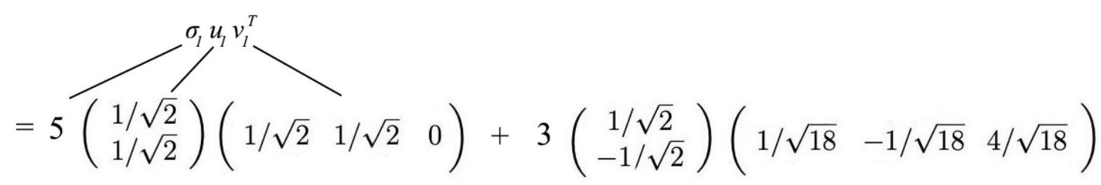
A=\left(\begin{array}{ccc}3 & 2 & 2 \\ 2 & 3 & -2\end{array}\right)

Uses of SVD

Moore–Penrose pseudoinverse

Suppose we want to solve a linear system

A x = b.

If A is invertible, the solution is

x = A^{-1} b.

But many matrices are not invertible:

• A may not be square,
• or it may have linearly dependent columns.

In this case, an exact solution may not exist. Instead, we look for the vector x that minimizes the least–squares error

|Ax-b|_2.

Among all least–squares solutions, we choose the one with smallest norm.

This motivates the Moore–Penrose pseudoinverse A^+, defined so that

x = A^+ b

is the minimum-norm least–squares solution.

Using the SVD

Take the singular value decomposition

A = U \Sigma V^T,

where

• U and V are orthogonal matrices,
• \Sigma is diagonal (possibly rectangular):

\Sigma = \begin{bmatrix} \sigma_1 &&&\\ & \ddots &&\\ && \sigma_r &&\\ &&& 0 \end{bmatrix}, \qquad \sigma_1 \ge \cdots \ge \sigma_r >0.

---

Normal equations

Least squares solutions satisfy the Normal equations

A^T A x = A^T b.

Substitute the SVD:

(V \Sigma^T U^T)(U \Sigma V^T)x = V \Sigma^T U^T b.

Since U^TU=I,

V \Sigma^T \Sigma V^T x = V \Sigma^T U^T b.

Multiply on the left by V^T:

\Sigma^T \Sigma V^T x = \Sigma^T U^T b.

Solve componentwise

\Sigma^T \Sigma V^T x = \Sigma^T U^T b.

We can write this componentwise as

\Sigma^T \Sigma \begin{bmatrix} \mathbf{v}_1^T \mathbf{x} \\ \mathbf{v}_2^T \mathbf{x} \\ \vdots \\ \mathbf{v}_n^T \mathbf{x} \end{bmatrix}= \Sigma^T \begin{bmatrix} \mathbf{u}_1^T \mathbf{b} \\ \mathbf{u}_2^T \mathbf{b} \\ \vdots \\ \mathbf{u}_n^T \mathbf{b} \end{bmatrix}.

Since both \Sigma^T and \Sigma^T\Sigma are diagonal, they just multiply each element by the corresponding singular value (or square):

\Sigma^T \Sigma V^T \mathbf{x} = \Sigma^T U^T \mathbf{b}

becomes

\begin{bmatrix} \sigma_1^2 \mathbf{v}_1^T \mathbf{x} \\ \sigma_2^2 \mathbf{v}_2^T \mathbf{x} \\ \vdots \\ \sigma_n^2 \mathbf{v}_n^T \mathbf{x} \\ \end{bmatrix} = \begin{bmatrix} \sigma_1\mathbf{u}_1^T \mathbf{b} \\ \sigma_2\mathbf{u}_2^T \mathbf{b} \\ \vdots \\ \sigma_n\mathbf{u}_n^T \mathbf{b} \end{bmatrix}.

In other words, we get a separate equation for each singular value \sigma_i:

\sigma_i^2 \mathbf{v}_i^T \mathbf{x} = \sigma_i (\mathbf{u}_i^T \mathbf{b}).

Case 1: \sigma_i \neq 0

\sigma_i^2 \mathbf{v}_i^T \mathbf{x} = \sigma_i (\mathbf{u}_i^T \mathbf{b}).

We can divide by \sigma_i^2:

\mathbf{v}_i^T \mathbf{x} = \frac{1}{\sigma_i} \mathbf{u}_i^T \mathbf{b}.

Case 2: \sigma_i = 0

\sigma_i^2 \mathbf{v}_i^T \mathbf{x} = \sigma_i (\mathbf{u}_i^T \mathbf{b}).

The equation becomes

0 = 0,

which imposes no constraint on y_i.

To obtain the minimum-norm solution, we choose \mathbf{x} to be orthogonal to \mathbf{v}_i, so that:

\mathbf{v}_i^T \mathbf{x} = 0.

Defining \Sigma^+

These two cases can be summarized by defining the pseudoinverse of \Sigma

\Sigma^+ = \begin{bmatrix} 1/\sigma_1 &&&\\ & \ddots &&\\ && 1/\sigma_r &\\ &&& 0 \end{bmatrix}.

That’s just replacing every non-zero singular value with its reciprocal.

Then the equation becomes

V^T \mathbf{x} = \Sigma^+ U^T \mathbf{b}.

The Moore–Penrose pseudoinverse

V^T \mathbf{x} = \Sigma^+ U^T \mathbf{b}.

Finally, we can multiply both sides on the left by V to get

\mathbf{x} = V \Sigma^+ U^T \mathbf{b}

The quantity V \Sigma^+ U^T is acting like an inverse here – it is called the Moore–Penrose pseudoinverse of A.

For any vector b,

\mathbf{x} = A^+ \mathbf{b}

is the minimum-norm solution to the least-squares problem.

Interpretation

\mathbf{x} = V \Sigma^+ U^T \mathbf{b}

The SVD reveals exactly what the pseudoinverse does:

• Each singular direction acts independently.
• Directions with \sigma_i>0 can be inverted.
• Directions with \sigma_i=0 contain information lost by A and cannot be recovered.

The pseudoinverse therefore

undoes the action of A wherever inversion is possible but ignores directions where information has been destroyed.

:::

Example

\begin{aligned} & A=\left[\begin{array}{ll} 1 & 1 \\ 1 & 1 \end{array}\right] \text { (singular, inverse does not exist) } \\ & A=U \Sigma V^{T}=\frac{1}{\sqrt{2}}\left[\begin{array}{rr} 1 & 1 \\ 1 & -1 \end{array}\right]\left[\begin{array}{rr} 2 & 0 \\ 0 & 0 \end{array}\right] \frac{1}{\sqrt{2}}\left[\begin{array}{rr} 1 & 1 \\ 1 & -1 \end{array}\right] \\ & A^{+}=V \Sigma^{+} U^{T}=\frac{1}{\sqrt{2}}\left[\begin{array}{rr} 1 & 1 \\ 1 & -1 \end{array}\right]\left[\begin{array}{cc} 1 / 2 & 0 \\ 0 & 0 \end{array}\right] \frac{1}{\sqrt{2}}\left[\begin{array}{rr} 1 & 1 \\ 1 & -1 \end{array}\right]=\frac{1}{4}\left[\begin{array}{ll} 1 & 1 \\ 1 & 1 \end{array}\right] \end{aligned}

Matrices as data

Example: Height and weight

A^T=\left[\begin{array}{rrrrrrrrrrrr}2.9 & -1.5 & 0.1 & -1.0 & 2.1 & -4.0 & -2.0 & 2.2 & 0.2 & 2.0 & 1.5 & -2.5 \\ 4.0 & -0.9 & 0.0 & -1.0 & 3.0 & -5.0 & -3.5 & 2.6 & 1.0 & 3.5 & 1.0 & -4.7\end{array}\right]

Why does A^T A appear? (Data interpretation)

Up to now, matrices like A^T A have appeared naturally during the construction of the SVD.

But suppose now that A is a data matrix.

What does A^T A actually represent?

Step 1 — Interpret A as data

Think of

• rows = observations (people)
• columns = variables (height, weight, etc.)

Each row is one data point in \mathbb{R}^p.

---

Step 2 — Center the data

Subtract the mean of each column so every variable has mean 0.

We now assume:

A \text{ is zero-centered.}

This assumption is the key bridge between linear algebra and statistics.

Step 3 — Examine one entry of A^T A

The (i,j) entry is

(A^T A)*{ij} = \sum*{k=1}^{n} A_{k i}A_{k j}.

This computation:

• multiplies variable i and variable j together,
• then adds across all observations.

That is exactly how we measure co-variation between variables.

---

Step 4 — The covariance matrix appears

For zero-centered data,

\Sigma = \frac{1}{n-1}A^T A

is the sample covariance matrix.

So the matrix that appeared in the SVD derivation is not mysterious at all:

A^T A measures how the variables vary together.

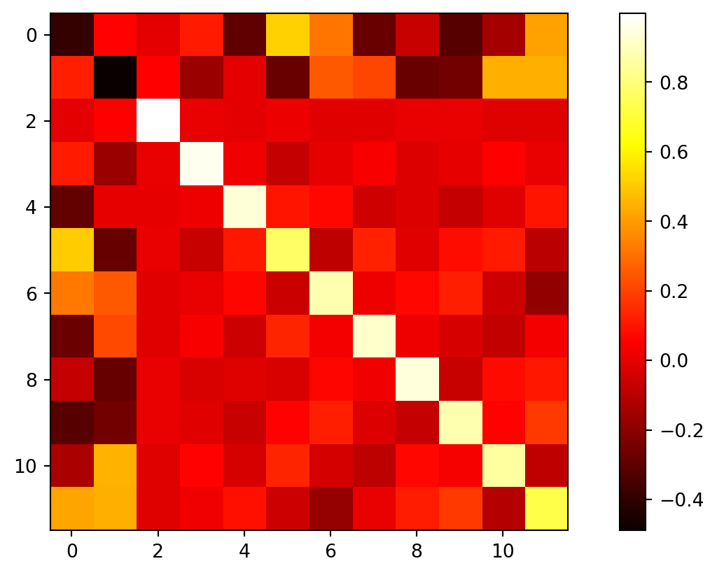
What do off-diagonal entries mean?

Look at a covariance matrix

\Sigma= \begin{bmatrix} \sigma_1^2 & c_{12} & \cdots c_{12} & \sigma_2^2 & \cdots \vdots & \vdots & \ddots \end{bmatrix}.

• The diagonal entries record how much each variable varies on its own.
• The off-diagonal entries measure how two variables move together.

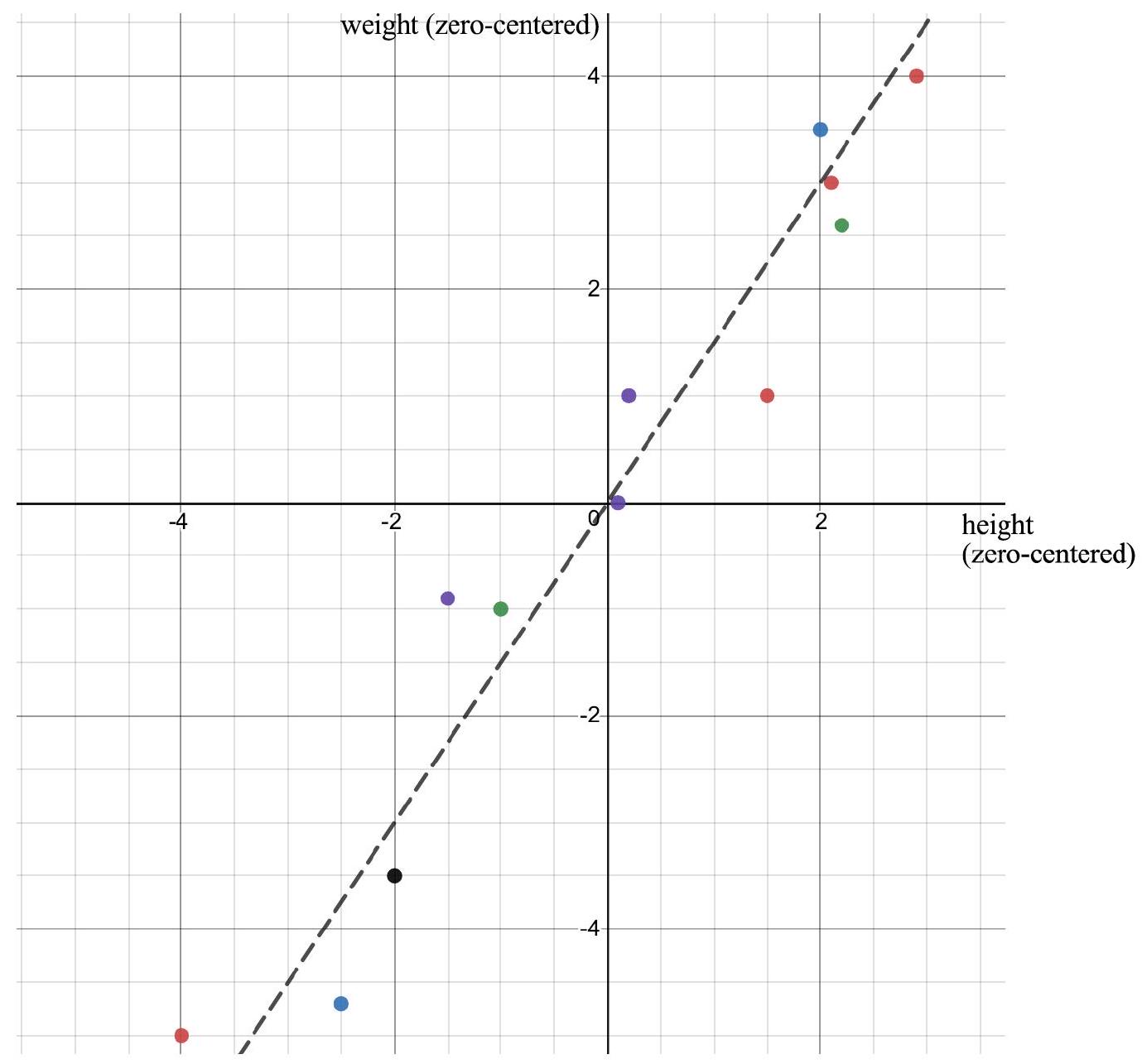
Heights and weights example

Let’s look at the (zero-centered) heights/weights dataset we’ve been using.

	height	weight
height	4.86	6.67
weight	6.67	9.74

The off-diagonal entry \Sigma_{12}= 6.67 is the covariance between height and weight.

• The positive value of the off-diagonal entry means that (in this dataset) when height increases, weight tends to increase too.

• Knowin the height of an individual lets us make a guess about their weight.

---

But what if we rotated the axes?

A tilted data cloud suggests we are using a coordinate system that is not aligned with the natural shape of the data.

Let’s rotate to new axes:

In the rotated coordinate system, moving along one new axis does not force movement along the other (the axes line up with the ellipse).

The covariance matrix in the rotated coordinates

Now compute the covariance matrix of the rotated data Y.

	axis 1	axis 2
axis 1	1.440778e+01	9.285502e-16
axis 2	9.285502e-16	1.940396e-01

This covariance matrix is diagonal (up to tiny numerical rounding), which means:

• along these rotated axes, the two coordinates are uncorrelated,
• the variation in the data separates cleanly into two independent directions.

A^T=\left[\begin{array}{rrrrrrrrrrrr}2.9 & -1.5 & 0.1 & -1.0 & 2.1 & -4.0 & -2.0 & 2.2 & 0.2 & 2.0 & 1.5 & -2.5 \\ 4.0 & -0.9 & 0.0 & -1.0 & 3.0 & -5.0 & -3.5 & 2.6 & 1.0 & 3.5 & 1.0 & -4.7\end{array}\right]

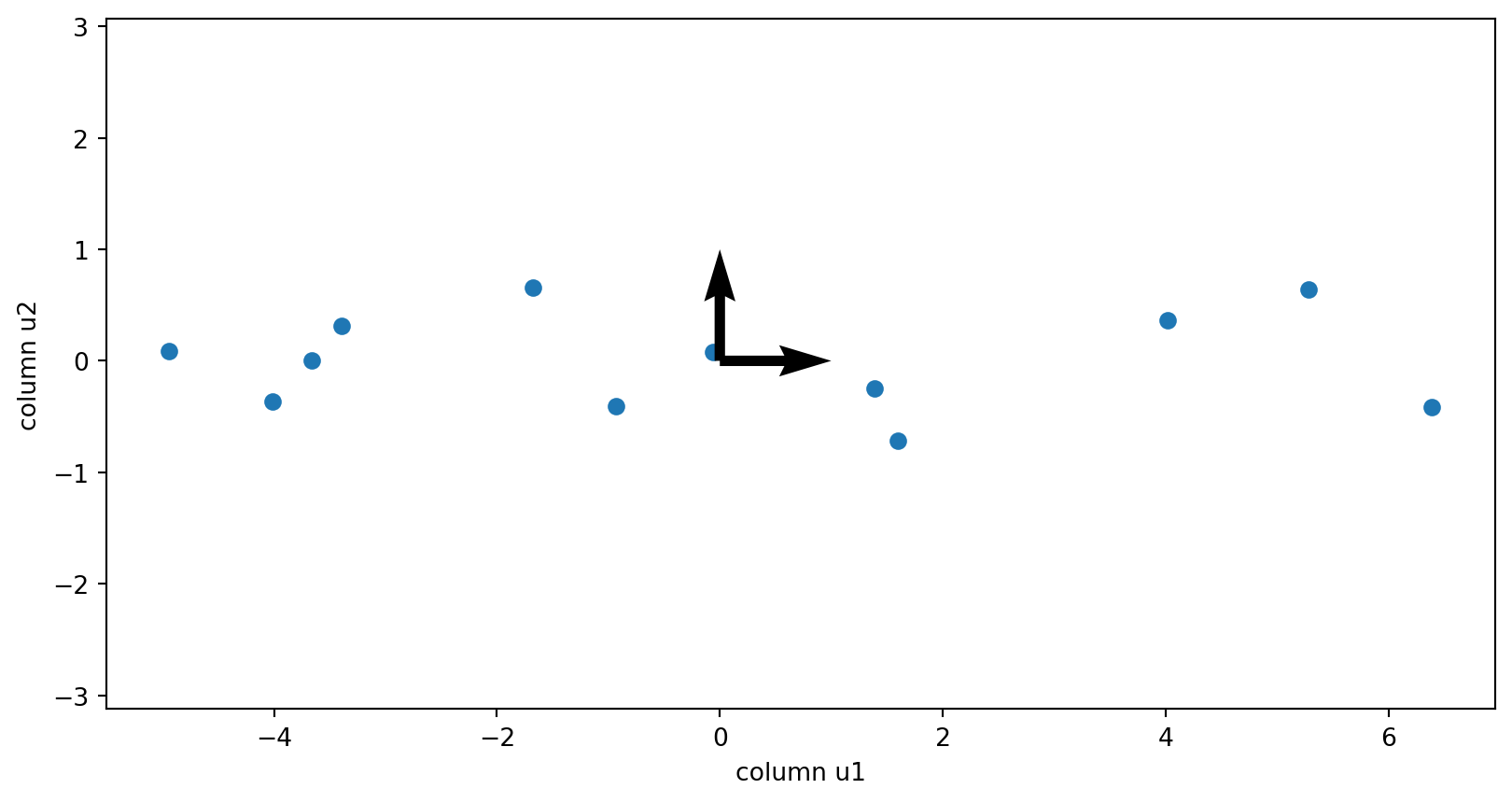
Plotting

The columns of the V matrix:

[[-0.57294952 -0.81959066]
 [ 0.81959066 -0.57294952]]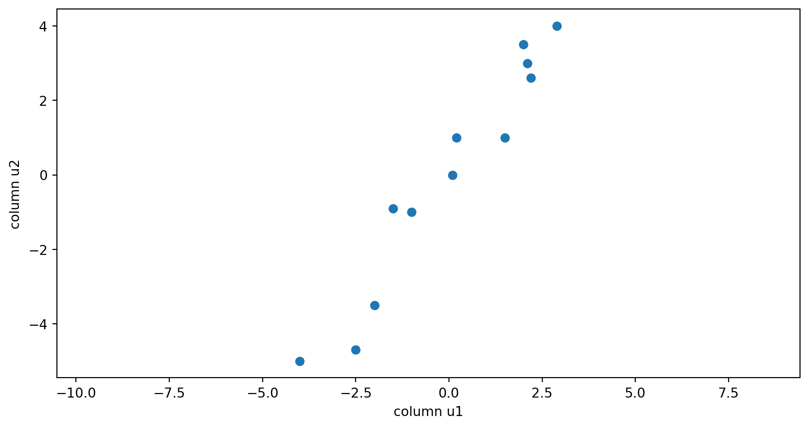

Walk through why these vectors are actually the eigenvectors of the covariance matrix.

Look at the covariance matrix: \text { Sample covariance } S^{2}=\frac{A^{T} A}{(\mathrm{n}-1)}=\frac{1}{11}\left[\begin{array}{rr} 53.46 & 73.42 \\ 73.42 & 107.16 \end{array}\right]

Calculate the covariance matrix times the eigenvector, by hand. See why it comes out the same, because it captures the results of the covariance matrix.

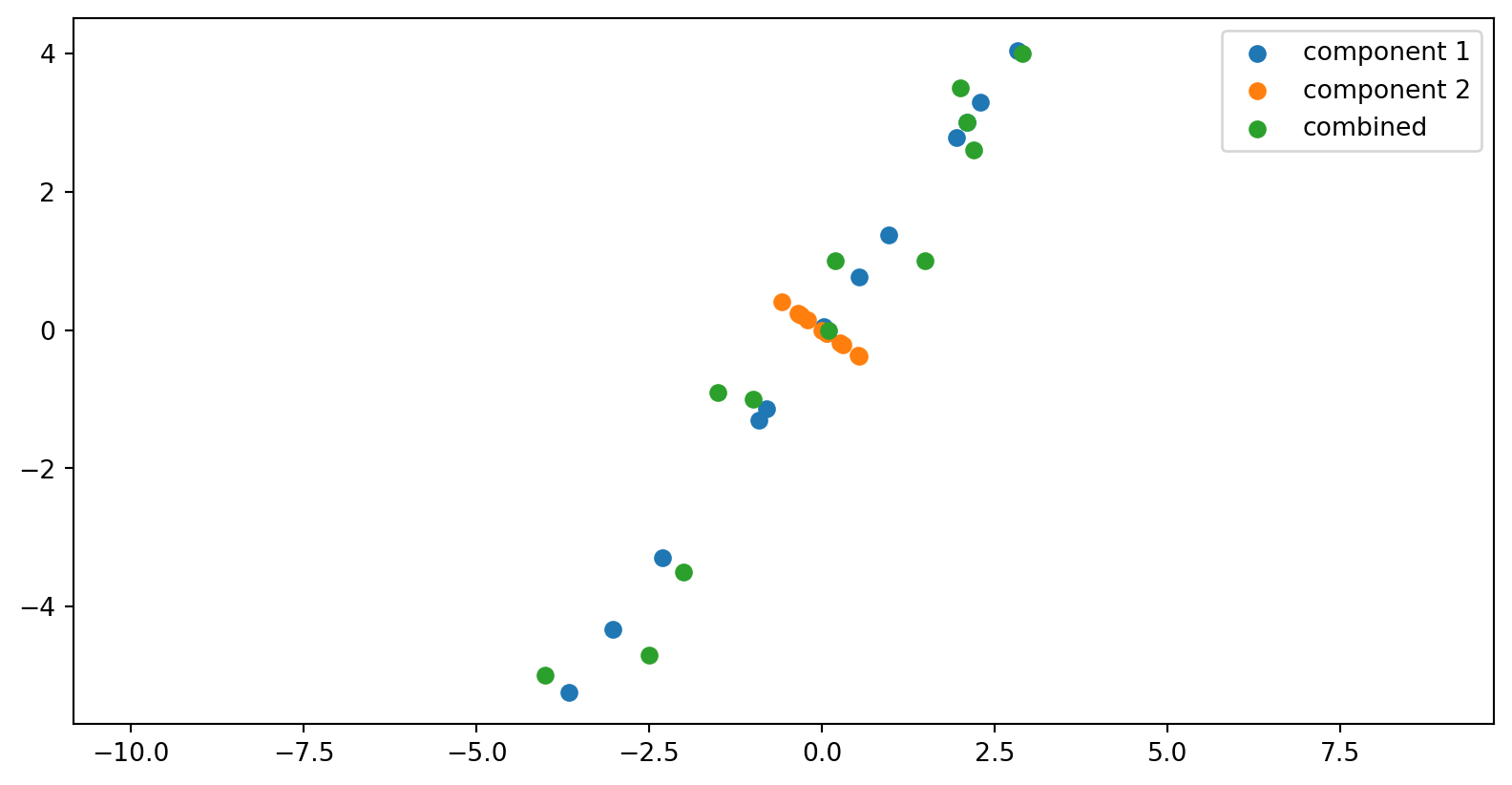
The components of the data matrix

The columns of the U matrix