Ch5 Lecture 4

Outline for today

• SVD on matrices of data
• SVD on images
• SVD in higher dimensions

SVD on matrices of data

Applying the SVD to tabular data; interpreting U and V; the outer-product sum.

Example: Height and weight

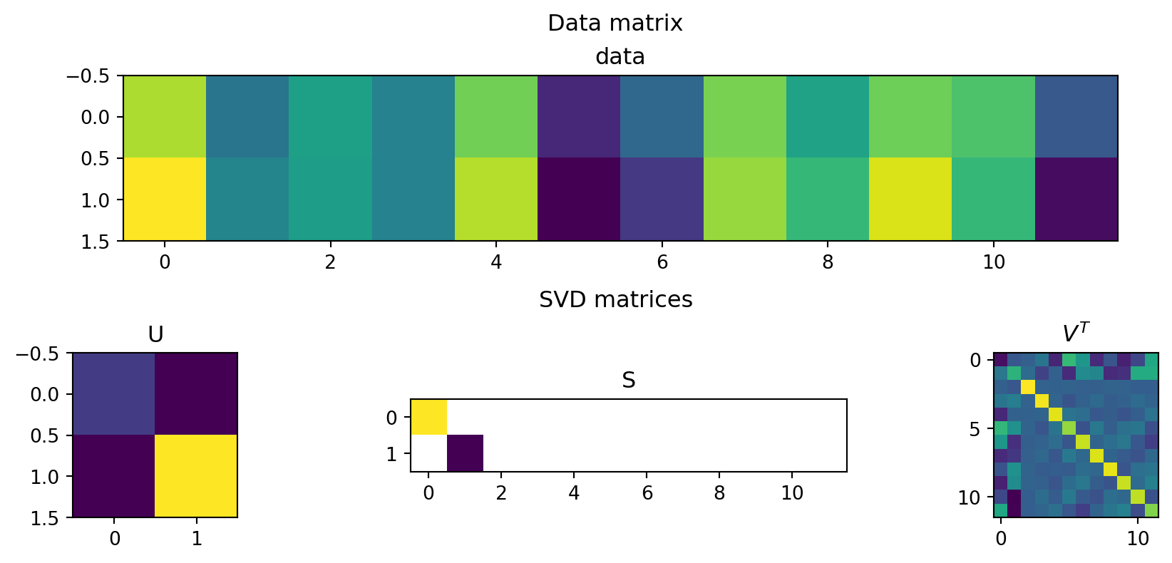
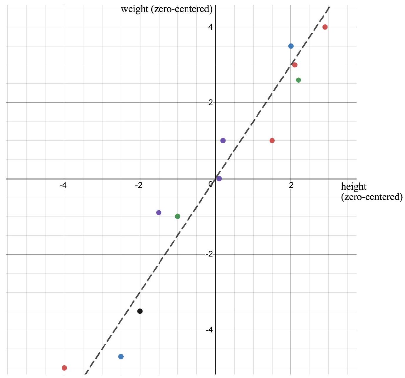
A^T= \begin{bmatrix} 2.9 & -1.5 & 0.1 & -1.0 & 2.1 & -4.0 & -2.0 & 2.2 & 0.2 & 2.0 & 1.5 & -2.5 \\ 4.0 & -0.9 & 0.0 & -1.0 & 3.0 & -5.0 & -3.5 & 2.6 & 1.0 & 3.5 & 1.0 & -4.7 \end{bmatrix}

Each column represents one person:

\begin{bmatrix} \text{height} \\ \text{weight} \end{bmatrix}.

• Rows = measurements (height, weight)
• Columns = individuals

---

---

Plotting

<Figure size 960x480 with 0 Axes>

The matrix U: directions among variables

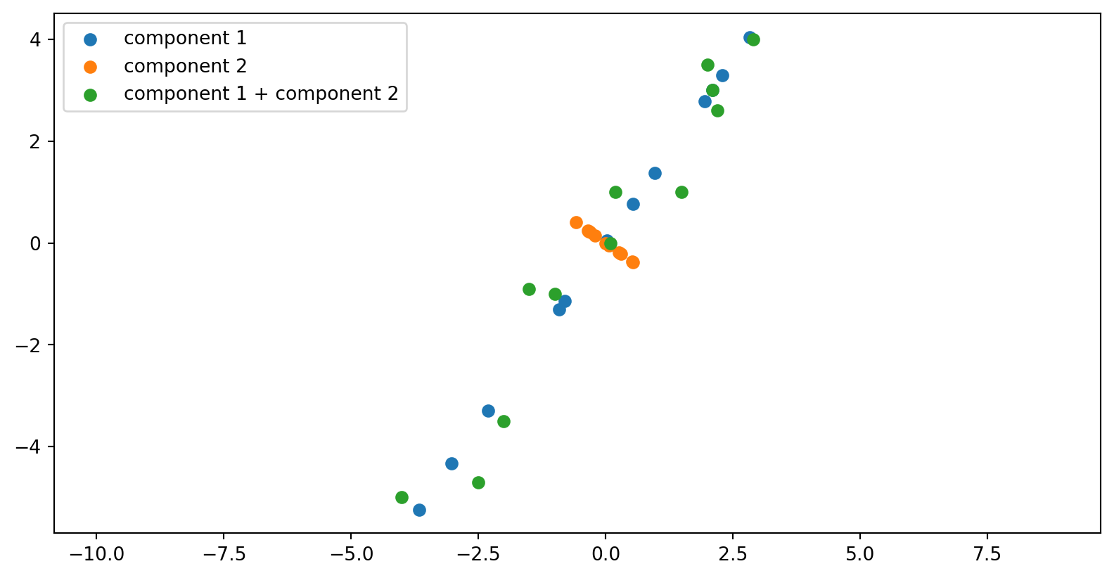
The columns of U live in height–weight space.

Each column u_i is a direction that can be drawn directly on the scatterplot.

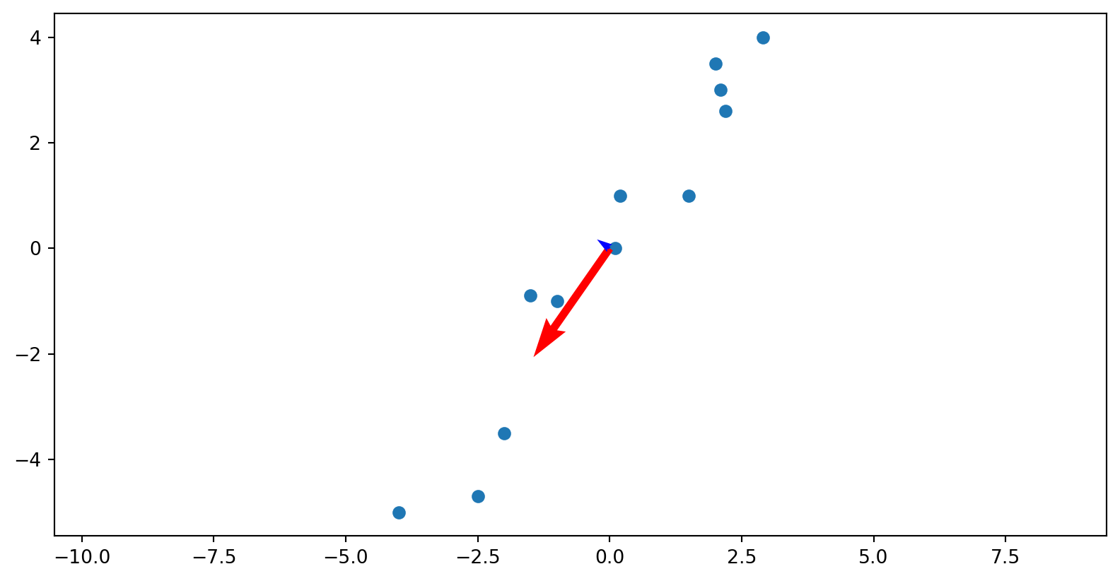
Each vector u_i answers:

If the data vary according to one underlying pattern, how do the measurements change?

Typical interpretation:

• u_1: height and weight increase together → overall body size direction.

• u_2: height increases while weight decreases (or vice versa) → body proportion differences.

So U provides an orthogonal coordinate system describing how measurements change.

---

The matrix V: patterns among people

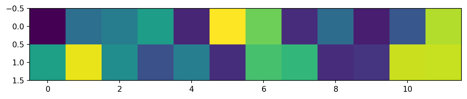
The matrix V lives in person space.

Each column v_i assigns a number to every person.

Each vector v_i tells us:

which people participate in a particular pattern of variation.

Interpretation:

• Large positive entry → that person strongly follows the pattern.
• Negative entry → participates in the opposite way.
• Near zero → little involvement.

Examples:

• The first pattern (in the first row) separates larger vs. smaller individuals.
• The second pattern (in the second row) contrasts tall–light vs. short–heavy people.

Because measurements live in a 2-dimensional space (height and weight), only two independent population patterns are needed.

---

Reconstructing the data

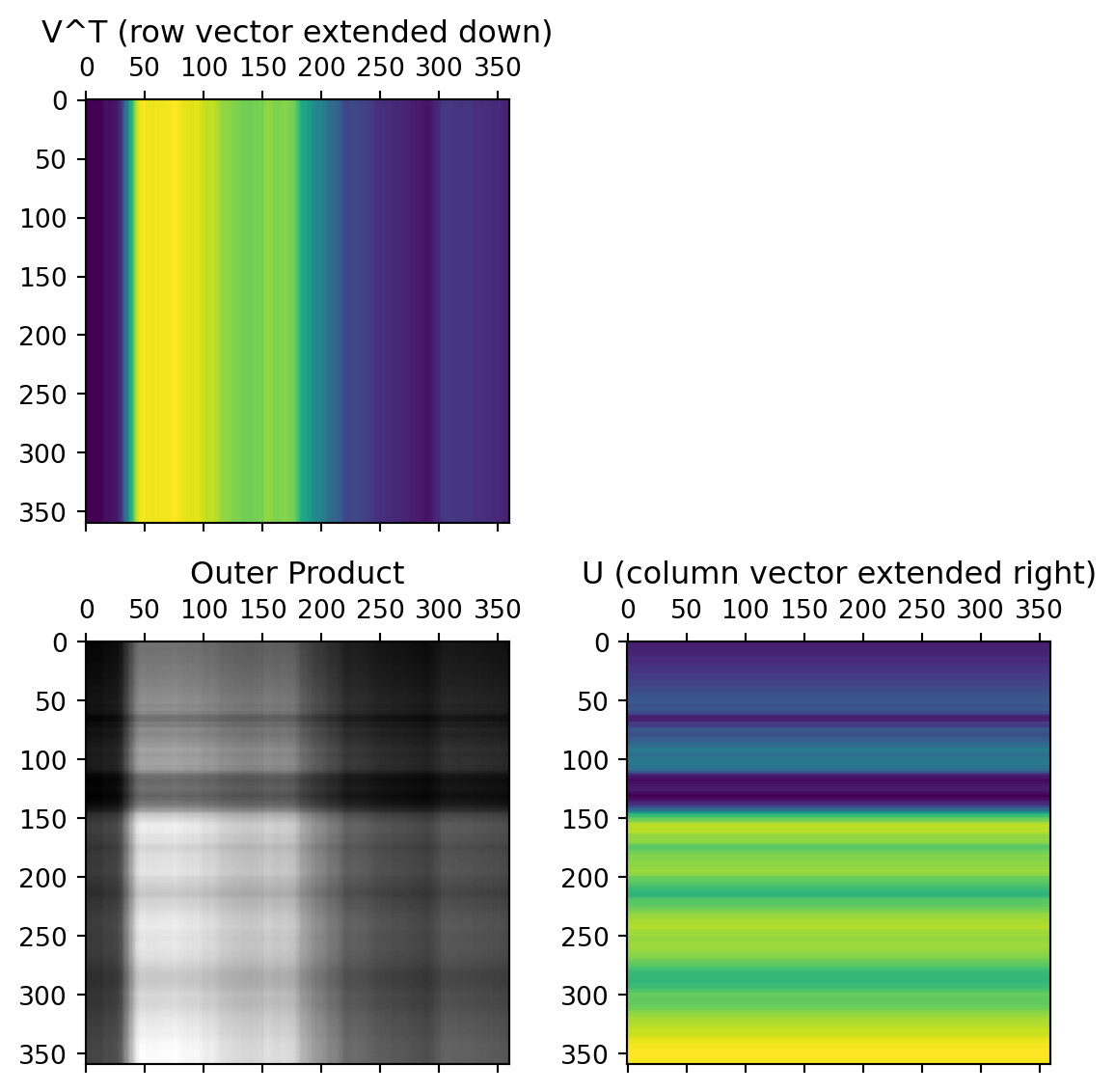
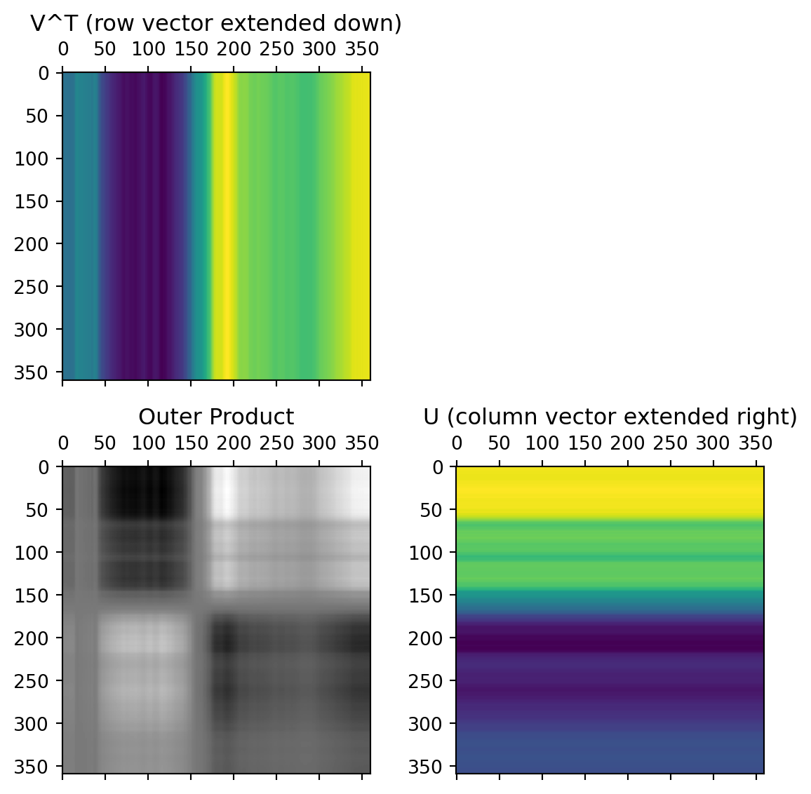
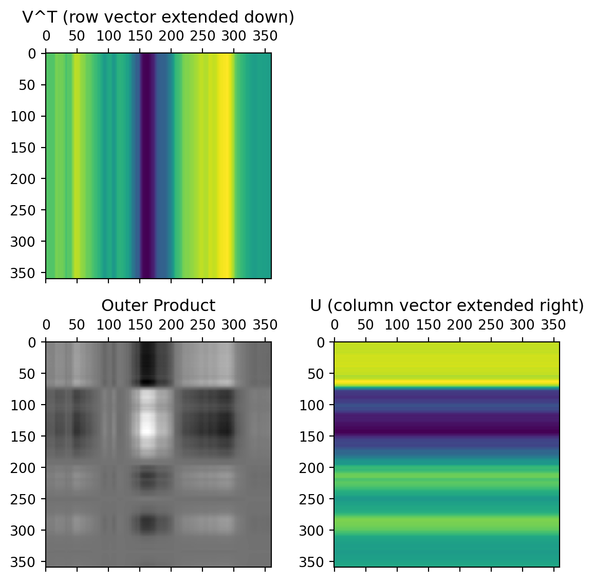
Using the first two rows of V^T, scaled by the singular values and rotated by U:

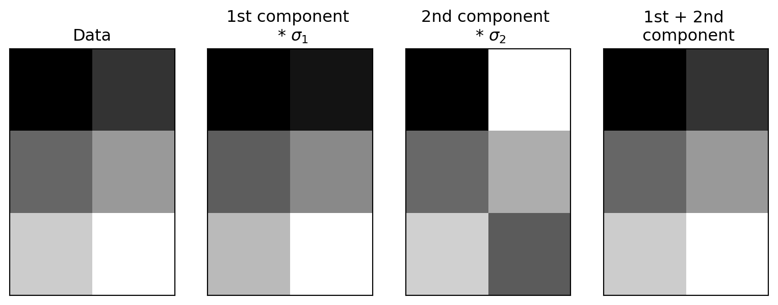
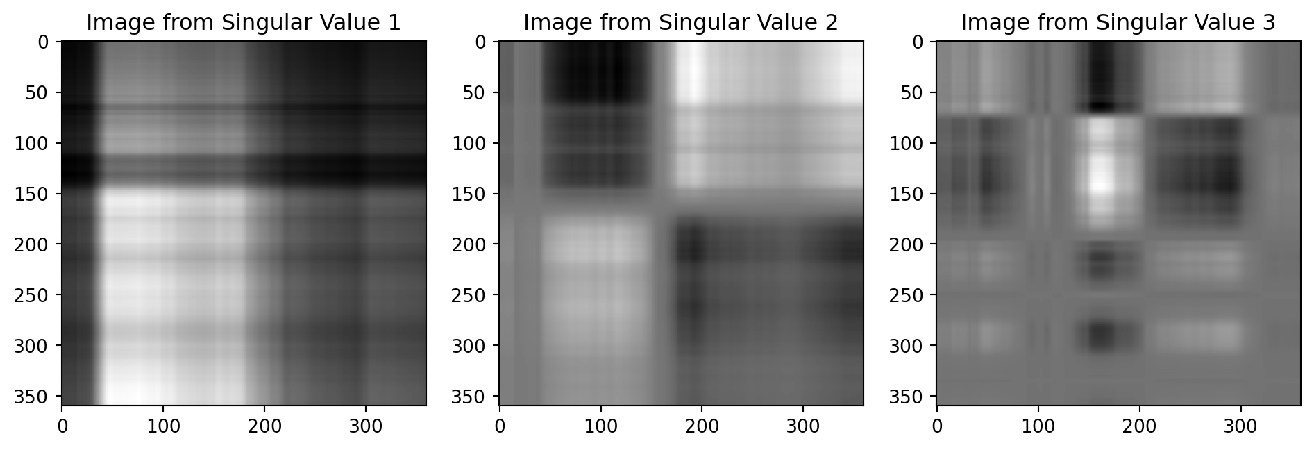
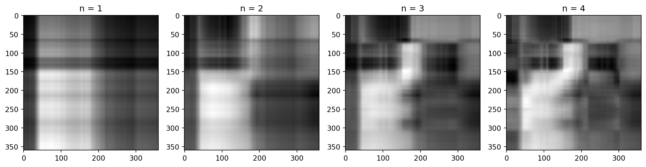
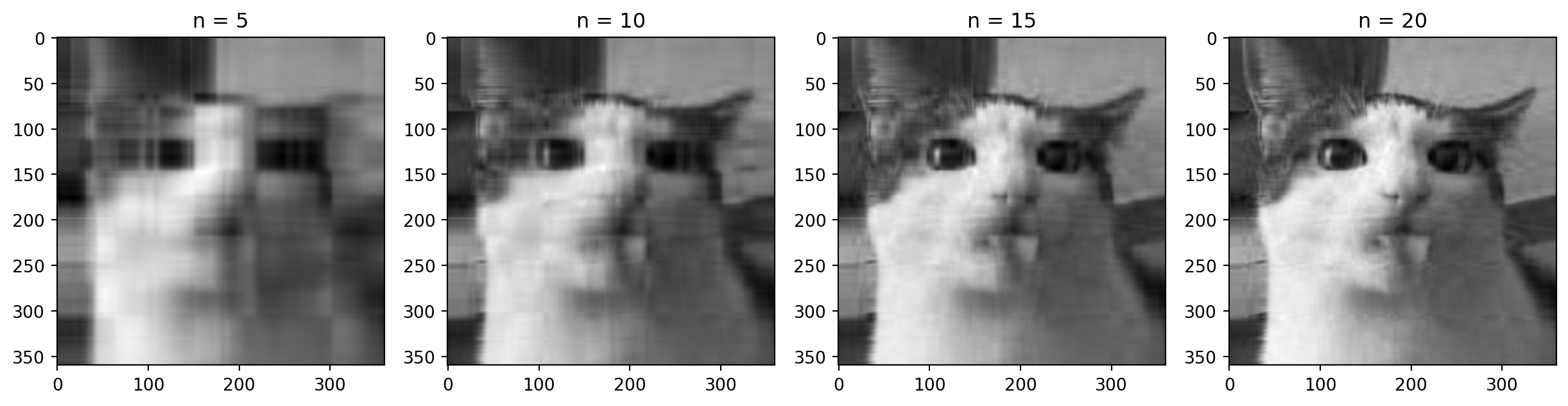
Each term of the SVD

A = U S V^\mathsf{T}

can be written as

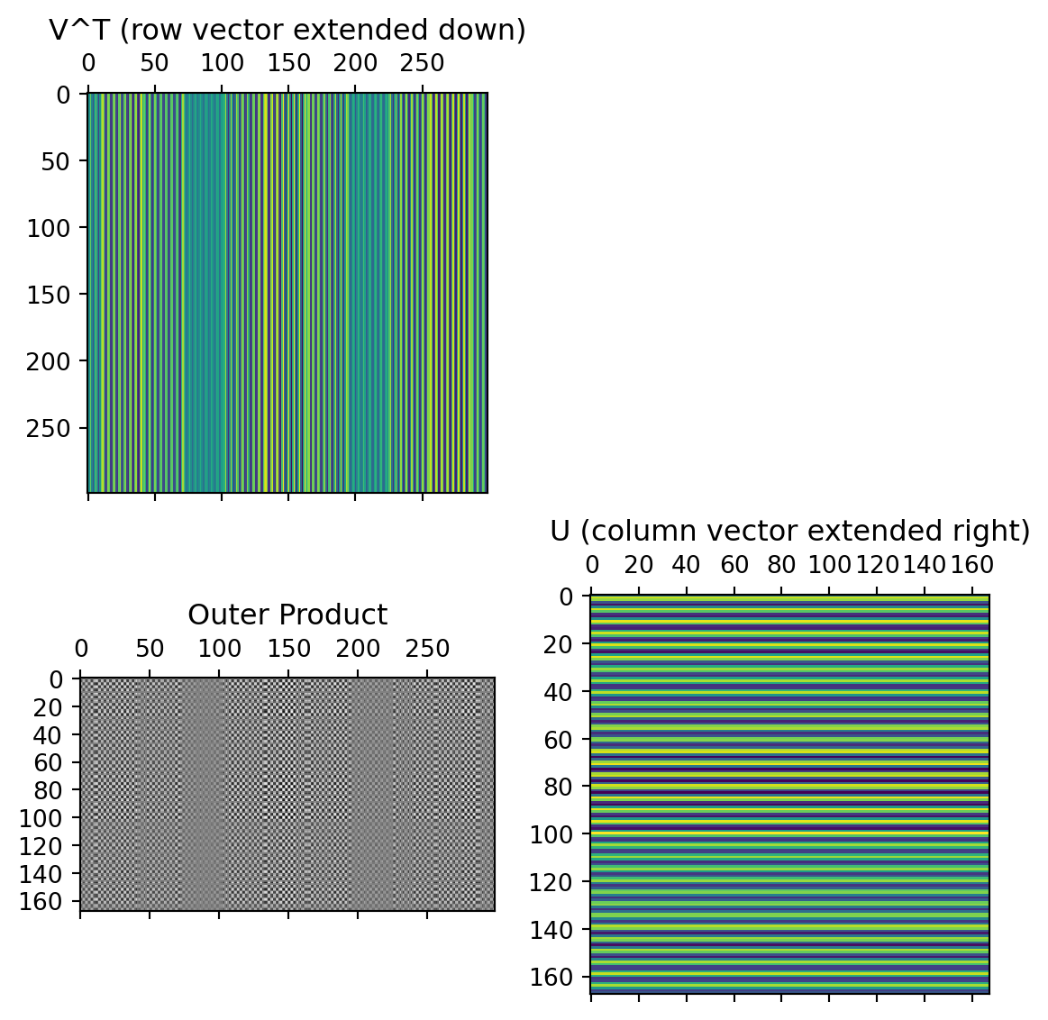
A = \sigma_1 u_1 v_1^\mathsf{T} + \dots + \sigma_r u_r v_r^\mathsf{T}.

Each component means:

• v_i: how much this individual participates in the pattern,
• u_i: how height and weight change,
• \sigma_i: how important this pattern is.

---

Skills

• Interpret the columns of U as directions of change in measurement space.

• Interpret the columns of V as independent patterns among individuals.

• Express the matrix as a sum of outer products \sigma_i \mathbf{u}_i \mathbf{v}_i^T. lls

• Interpret the columns of U as capturing relationships between rows of the data matrix

• Interpret the rows of V^T as capturing relationships between columns

• Express the matrix as a sum of outer products \sigma_i \mathbf{u}_i \mathbf{v}_i^T

SVD on images

SVD for image compression; left/right singular vectors; color images; PCA as truncated SVD.

Motivation: a cat

Dimensions of the decomposition

What are the dimensions of the decompositions for an image?

U, S, Vt = np.linalg.svd(image, full_matrices=False)
print(f'The shape of U is {U.shape}, the shape of S is {S.shape}, the shape of V is {Vt.shape}')

The shape of U is (360, 360), the shape of S is (360,), the shape of V is (360, 360)

What’s going on here? Walk through the way the rows and columns of U and V are used to reconstruct the image.

• U is a matrix that captures the relationships between the rows of the image. It mimics the columns.
• V is a matrix that captures the relationships between the columns of the image. It mimics the rows.
• We can interpret the singular values as the strength of the relationships captured by U and V
• The first columns of U and V capture the strongest relationships

Left singular values, corresponding to U, are the eigenvalues of AA^T. For an image, AA^T is the covariance matrix of the rows of A.

Right singular values are the eigenvalues of A^{T}A. For an image, A^TA is the covariance matrix of the columns of A.

Simple example

Walk through how the right singular vector looks a lot like the columns, and the left singular vector looks a lot like the rows.

Reconstructing our matrix

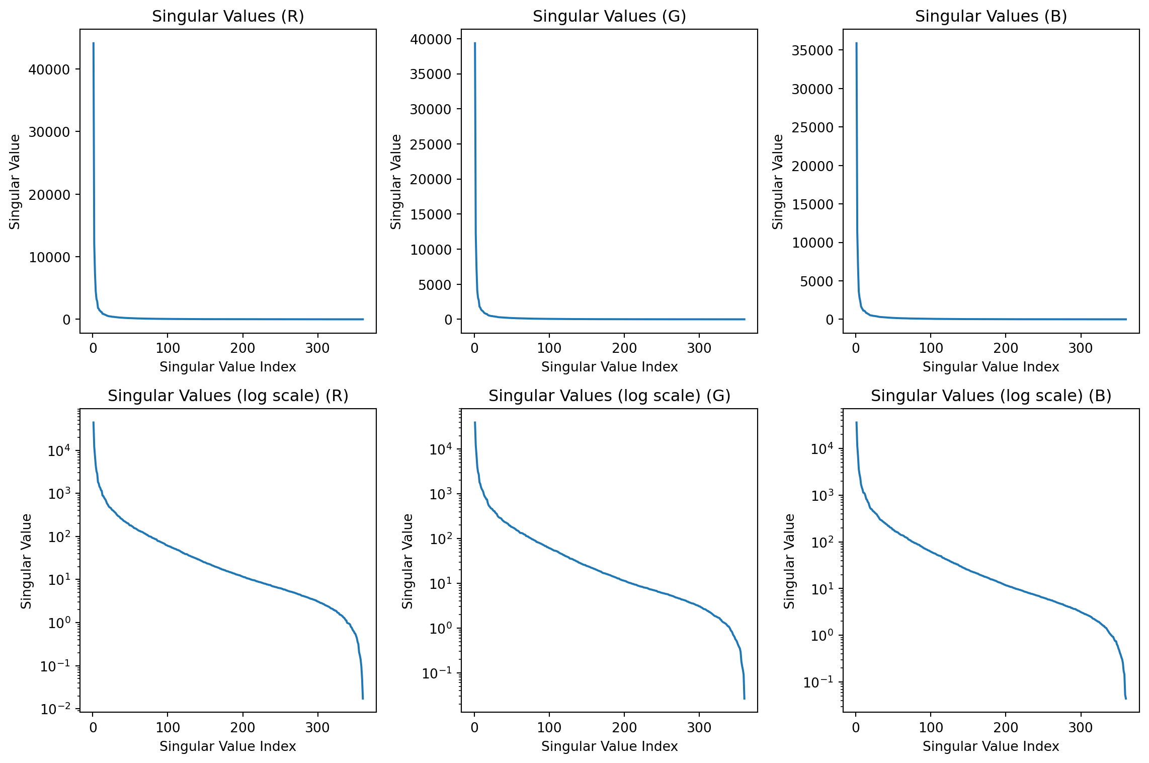
How much of the variance is captured by the first two components?

The variance captured by each component is the sum of the squares of the singular values divided by the sum of the squares of all the singular values.

Back to the cat

First Singular Value

Second Singular Value

Third Singular Value

Adding them up

Color images

# SVD for each channel
U_R, S_R, Vt_R = np.linalg.svd(R, full_matrices=False)
U_G, S_G, Vt_G = np.linalg.svd(G, full_matrices=False)
U_B, S_B, Vt_B = np.linalg.svd(B, full_matrices=False)

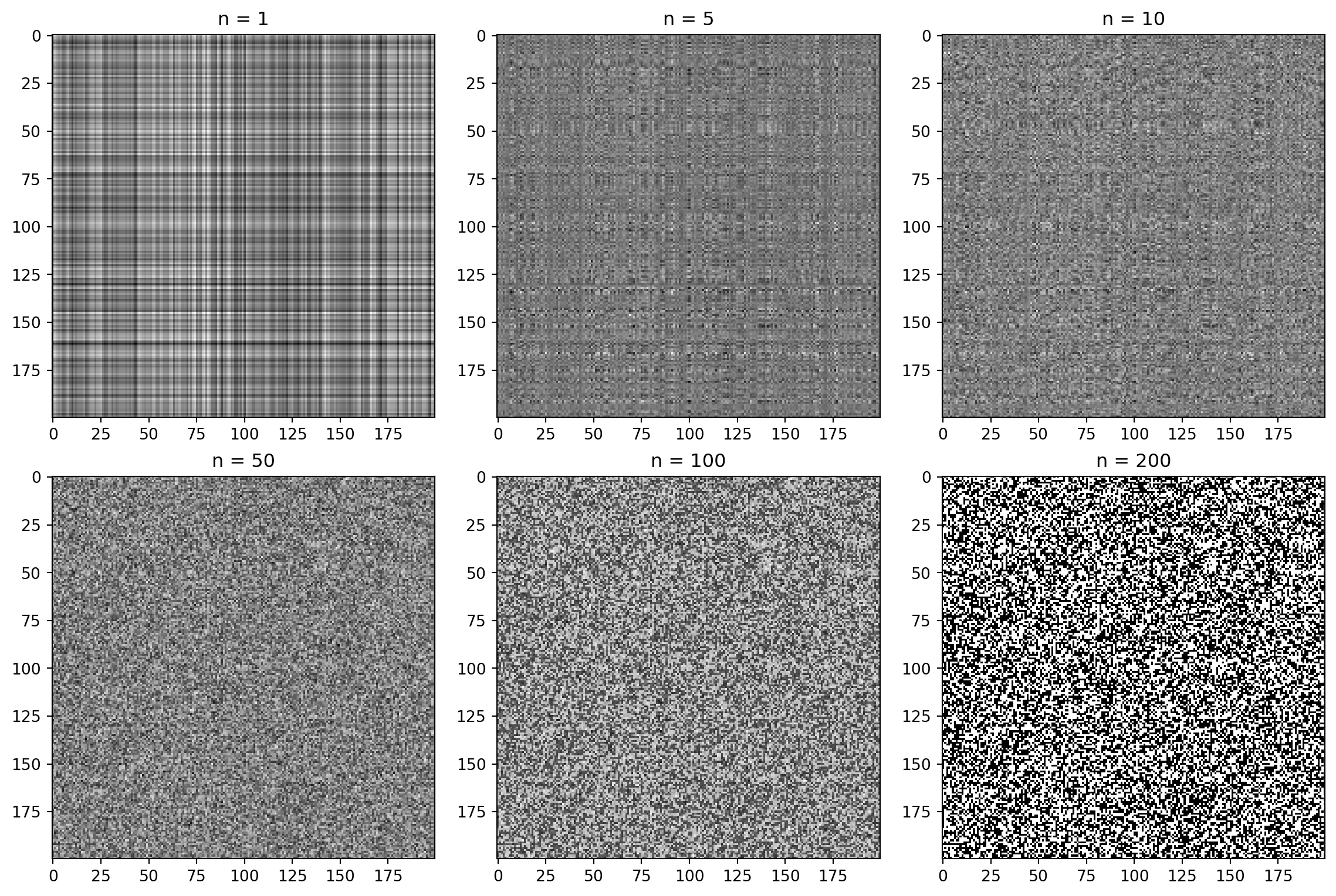
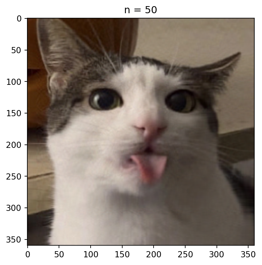
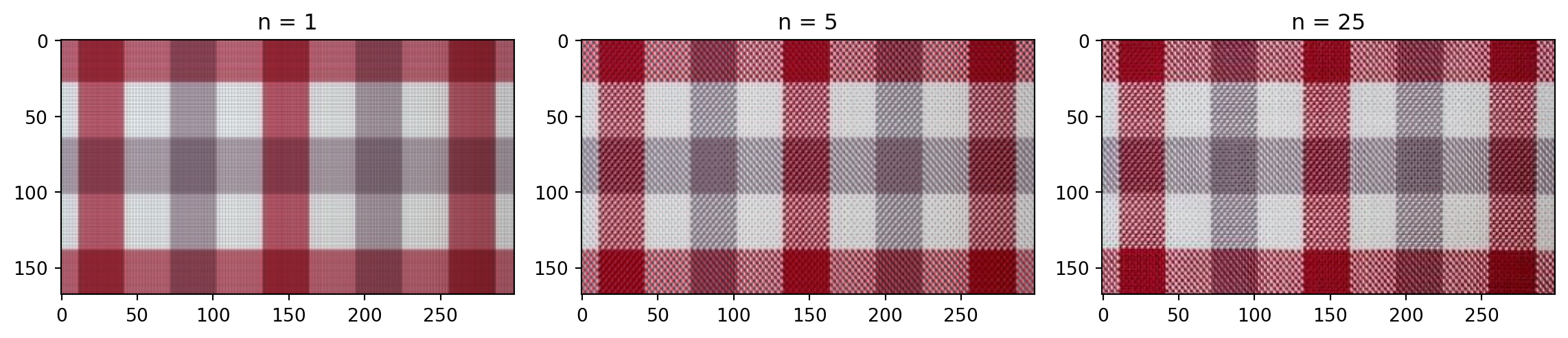
n = 50  # rank approximation parameter
R_compressed = np.matrix(U_R[:, :n]) * np.diag(S_R[:n]) * np.matrix(Vt_R[:n, :])
G_compressed = np.matrix(U_G[:, :n]) * np.diag(S_G[:n]) * np.matrix(Vt_G[:n, :])
B_compressed = np.matrix(U_B[:, :n]) * np.diag(S_B[:n]) * np.matrix(Vt_B[:n, :])

# Combining the compressed channels
compressed_image = cv2.merge([np.clip(R_compressed, 1, 255), np.clip(G_compressed, 1, 255), np.clip(B_compressed, 1, 255)])
compressed_image = compressed_image.astype(np.uint8)
plt.imshow(compressed_image)
plt.title('n = %s' % n)
plt.show()

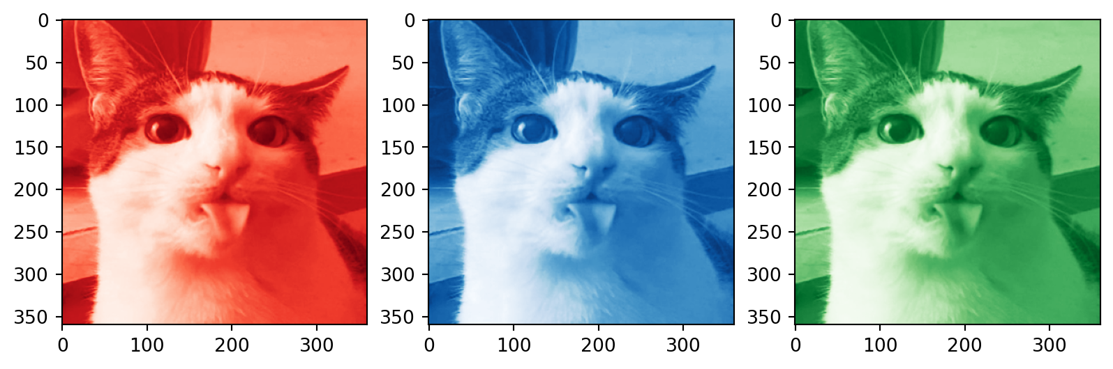
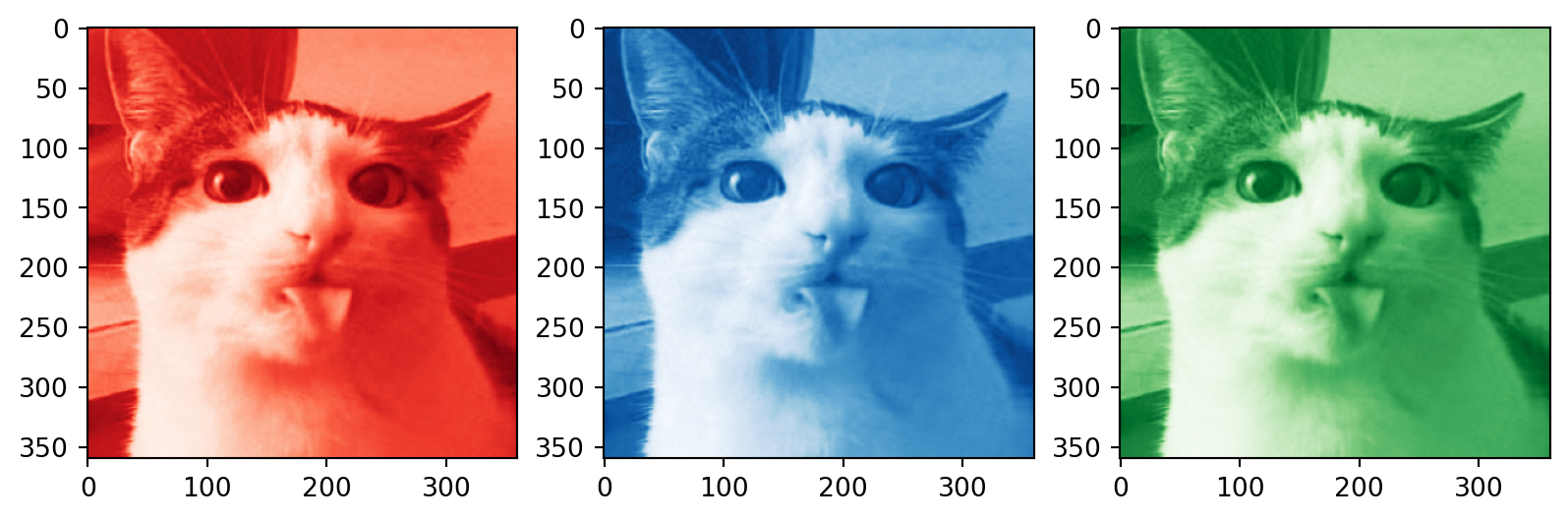
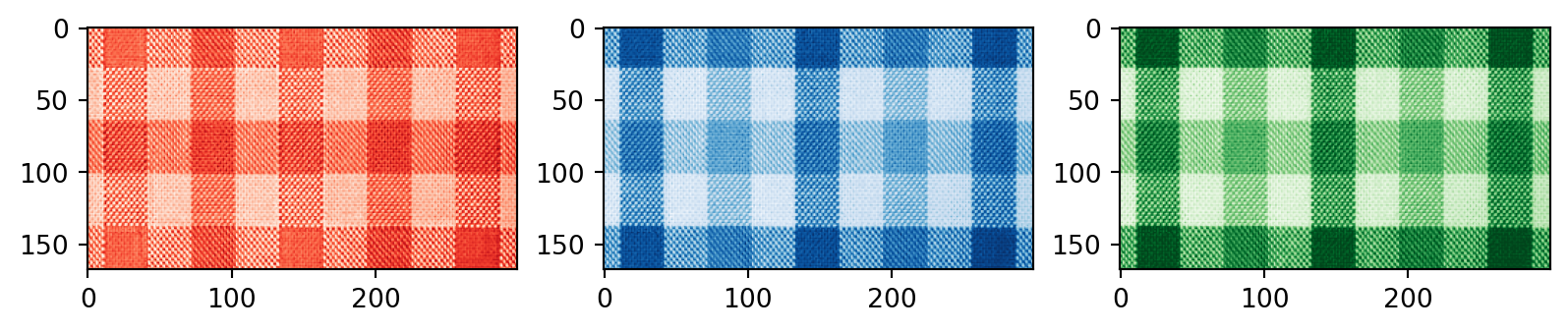
# Plotting the compressed RGB channels
plt.subplot(1, 3, 1)
plt.imshow(R_compressed, cmap='Reds_r')
plt.subplot(1, 3, 2)
plt.imshow(B_compressed, cmap='Blues_r')
plt.subplot(1, 3, 3)
plt.imshow(G_compressed, cmap='Greens_r')
plt.show()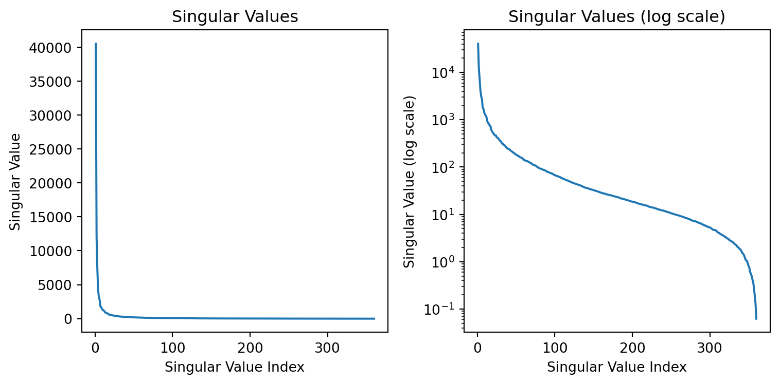

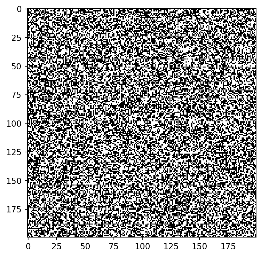
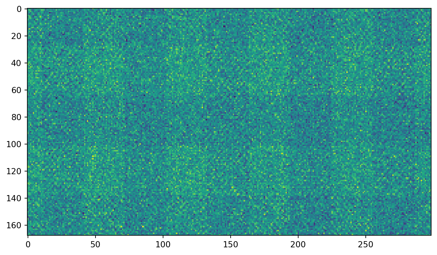
How many singular values to keep?

Different sorts of images

Just plain noise:

noise = np.random.randint(0,2,size=(200,200))
plt.imshow(noise, cmap='gray')

Why doesn’t this work?

Plaid shirt

What do we predict for how well the SVD will work on this image?

Singular values

Individual components

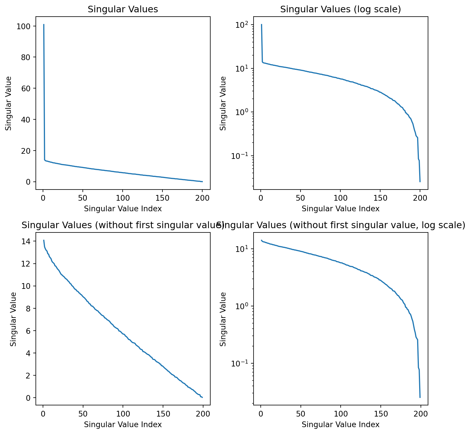
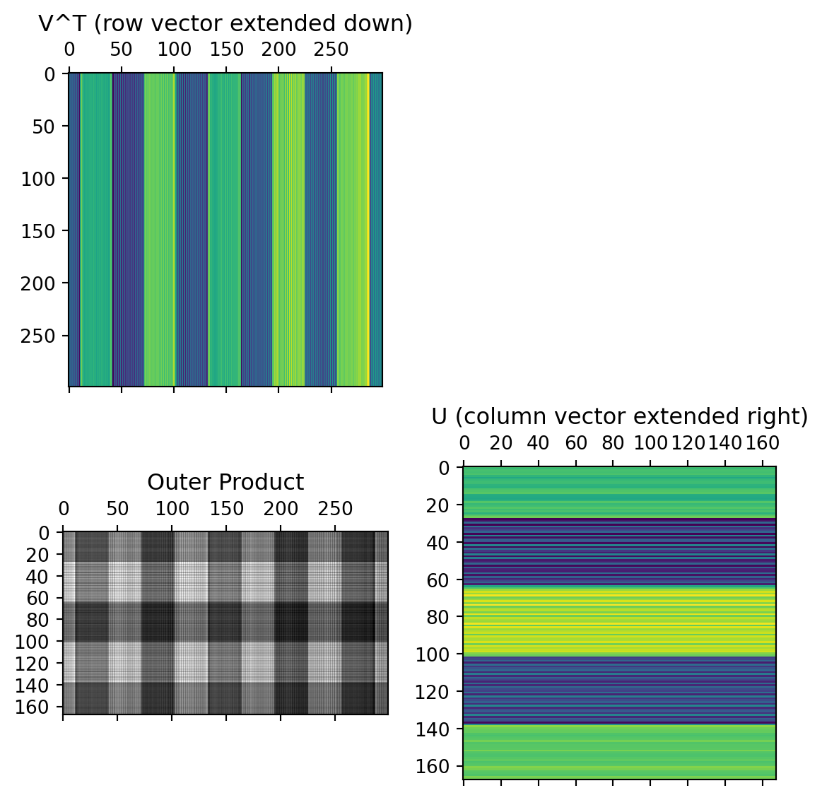
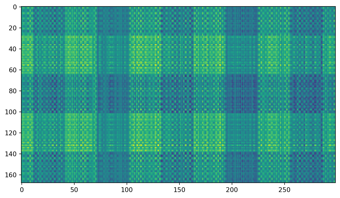
First component:

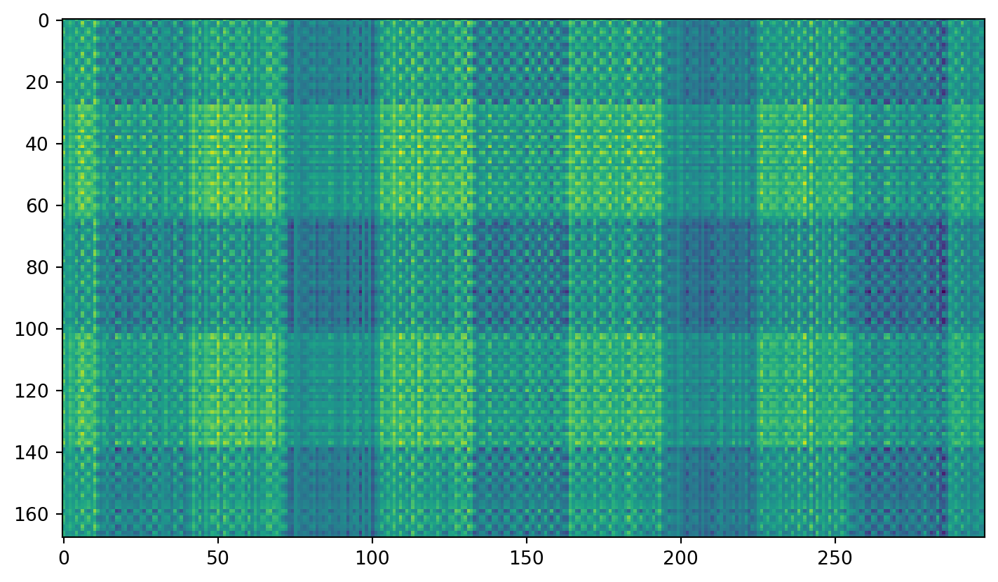
Second component:

Using “PCA” from sklearn

This is just an easier way to implement taking these first few components…

from sklearn.decomposition import PCA
pca = PCA(n_components=2)
pca.fit(R) # fit the model -- compute the matrices
transformed = pca.transform(R) # transform the data
print(f'The shape of the image is {R.shape}, and the shape of the compressed image is {transformed.shape}')
plt.imshow(transformed.T)

The shape of the image is (168, 299), and the shape of the compressed image is (168, 2)

plt.imshow(pca.inverse_transform(transformed))

Try adding noise…

alpha = 10
R_noisy = R + np.random.normal(0, 10, R.shape)*alpha
plt.imshow(R_noisy)

Now clean it up with PCA:

pca = PCA(n_components=2)
pca.fit(R_noisy)
plt.imshow(pca.inverse_transform(pca.transform(R_noisy)))

Skills

• Compute the SVD of an image matrix and interpret U, S, V
• Reconstruct an image from the first n singular value components
• Apply SVD to color images (per channel)
• Use PCA as a convenient truncated SVD; interpret variance captured

SVD in higher dimensions

PCA on high-dimensional data (faces); low-rank reconstruction; connection to SVD.

Faces

from sklearn.datasets import fetch_lfw_people
faces = fetch_lfw_people(min_faces_per_person=60)


# display a few of the faces, along with their names
fig, ax = plt.subplots(3, 4)
for i, axi in enumerate(ax.flat):
    axi.imshow(faces.images[i], cmap='bone')
    axi.set(xticks=[], yticks=[],
            xlabel=faces.target_names[faces.target[i]]) 

print(f'The shape of the faces dataset is {faces.images.shape}')

The shape of the faces dataset is (1348, 62, 47)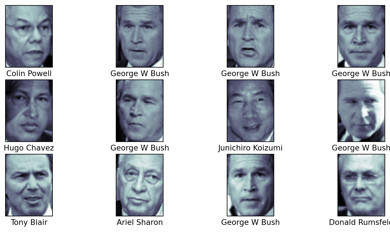

How is this dataset structured? What are the dimensions of the data? What do the rows and columns represent? Can we use our normal SVD, or do we need to extend it?

PCA on faces

pca = PCA(150, svd_solver='randomized', random_state=42)
pca_small = PCA(10, svd_solver='randomized', random_state=42)
pca_very_small = PCA(2, svd_solver='randomized', random_state=42)
pca.fit(faces.data)
pca_small.fit(faces.data)
pca_very_small.fit(faces.data)

PCA(n_components=2, random_state=42, svd_solver='randomized')

In a Jupyter environment, please rerun this cell to show the HTML representation or trust the notebook.
On GitHub, the HTML representation is unable to render, please try loading this page with nbviewer.org.

This treatment from here

Reconstructions

Really cool demo of SVD image compression: https://timbaumann.info/svd-image-compression-demo/

Skills

• Apply PCA to high-dimensional data (e.g., faces) and interpret components
• Reconstruct data from a low-rank PCA approximation
• Recognize PCA as truncated SVD on mean-centered data

Now you

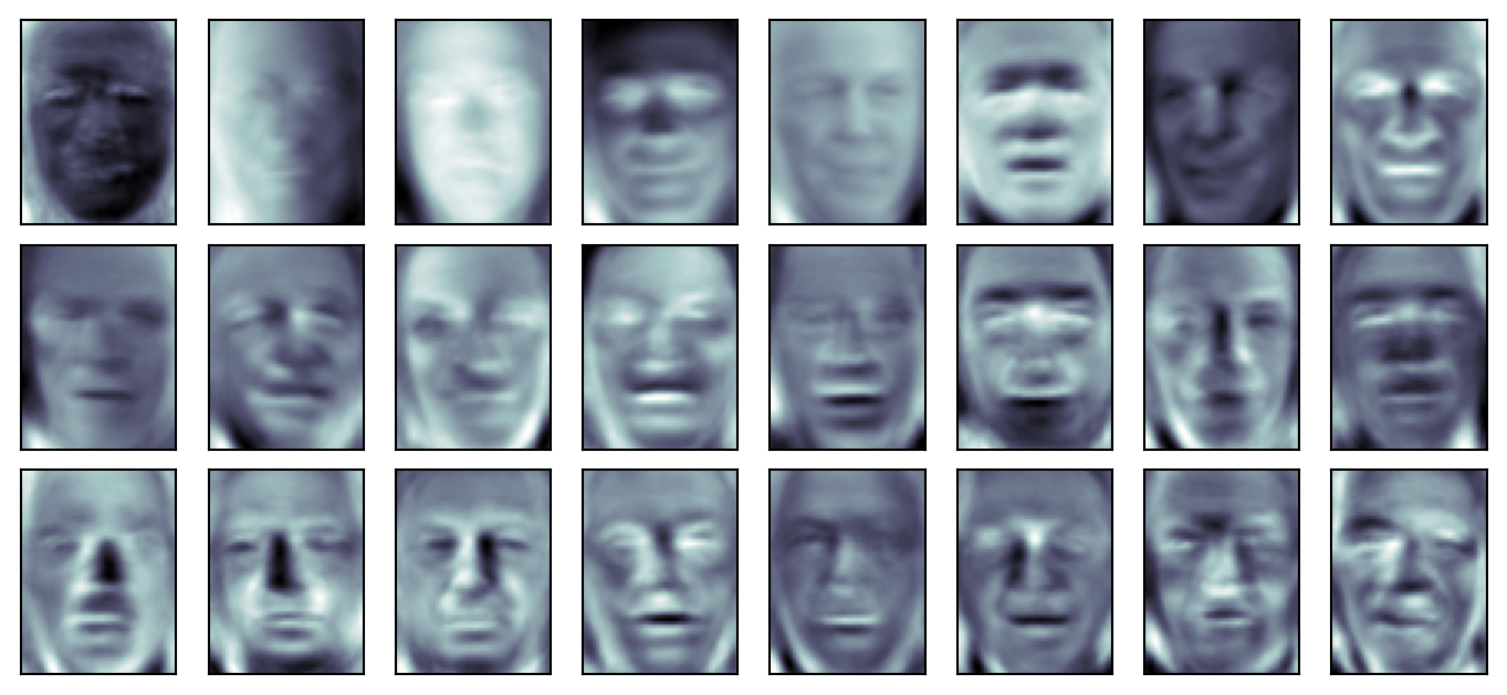
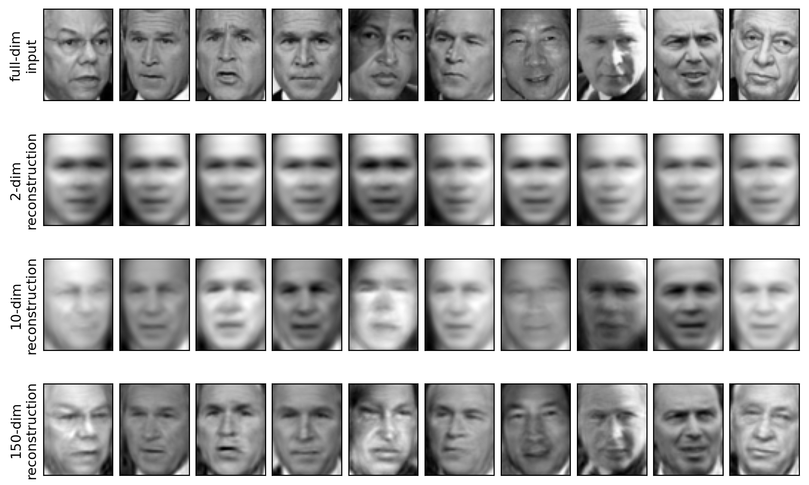
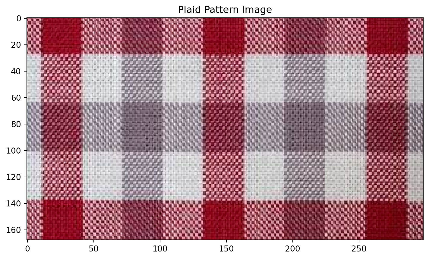
Code up your own image compression using SVD and show the left and right singular vectors, the singular values, and the reconstructed images.

Share with the class!