Ch3 Lecture 1

Linear Independence

Why care about linear independence?

Tells us whether vectors provide “new information” or redundantly describe the same directions.
Connects to solving systems: linearly independent columns \Rightarrow at most one solution to A\mathbf{x}=\mathbf{b}.

Linear Independence

The vectors \mathbf{v}_{1}, \mathbf{v}_{2}, \ldots, \mathbf{v}_{n} are linearly dependent if there exist scalars c_{1}, c_{2}, \ldots, c_{n}, not all zero, such that

c_{1} \mathbf{v}_{1}+c_{2} \mathbf{v}_{2}+\cdots+c_{n} \mathbf{v}_{n}=\mathbf{0}

Otherwise, the vectors are called linearly independent.

Linear Independence in matrix form

Let’s see if we can rewrite the condition for linear dependence in matrix form.

c_{1} \mathbf{v}_{1}+c_{2} \mathbf{v}_{2}+\cdots+c_{n} \mathbf{v}_{n}=\mathbf{0}

Define:

matrix A=\left[\mathbf{v}_{1}, \mathbf{v}_{2}, \mathbf{v}_{3}\right]
vector \mathbf{c}=\left(c_{1}, c_{2}, c_{3}\right).

Then:

c_{1} \mathbf{v}_{1}+c_{2} \mathbf{v}_{2}+c_{3} \mathbf{v}_{3}=\left[\mathbf{v}_{1}, \mathbf{v}_{2}, \mathbf{v}_{3}\right]\left[\begin{array}{l} c_{1} \\ c_{2} \\ c_{3} \end{array}\right]=A \mathbf{c}

Therefore, the vectors \mathbf{v}_1, \mathbf{v}_2, \ldots, \mathbf{v}_n are linearly dependent if there exists a nontrivial (nonzero) solution to [\mathbf{v}_1, \mathbf{v}_2, \ldots, \mathbf{v}_n] \mathbf{c}=\mathbf{0}.

Alternatively, we can say that the columns of A are linearly dependent if there exists a nontrivial solution to A \mathbf{c}=\mathbf{0}.

The relationship between linear independence and invertibility

The columns of A are linearly dependent if there exists a nontrivial solution to A \mathbf{c}=\mathbf{0}.

Conversely, the columns of A are linearly independent if \mathbf{c}=0 is the only solution to A \mathbf{c}=\mathbf{0}.

If the matrix A happens to be square, we can make a connection to invertibility.

Remember from the Day 5 lecture, one way of stating that a matrix is invertible (non-singular) is if \mathbf{c}=0 is the only solution to A \mathbf{c}=\mathbf{0}.

Therefore, for an n \times n matrix A, the columns are linearly independent if and only if A is invertible (non-singular).

Checking for Linear Independence

Is this set of vectors linearly independent?

\left[\begin{array}{l}1 \\ 1 \\ 0\end{array}\right],\left[\begin{array}{l}0 \\ 1 \\ 1\end{array}\right],\left[\begin{array}{r}1 \\ -1 \\ -2\end{array}\right]

Goal: find some set of scalars c_{1}, c_{2}, c_{3}, not all zero, such that c_{1} \mathbf{v}_{1}+c_{2} \mathbf{v}_{2}+c_{3} \mathbf{v}_{3}=\mathbf{0}.

How can we do this? We could just guess at some values for c_1, c_2, c_3 and see if they work…

Indeed, we can see that c_1 = -1, c_2 = 2, c_3 = 1 works:

\begin{gathered} -1 \left[\begin{array}{l}1 \\ 1 \\ 0\end{array}\right] + 2 \left[\begin{array}{l}0 \\ 1 \\ 1\end{array}\right] + 1 \left[\begin{array}{r}1 \\ -1 \\ -2\end{array}\right] \\ = \left[\begin{array}{l} -1 \times 1 + 2 \times 0 + 1 \times 1 \\ -1 \times 1 + 2 \times 1 + 1 \times (-1) \\ -1 \times 0 + 2 \times 1 + 1 \times (-2) \end{array}\right] = \left[\begin{array}{l} -1 + 0 + 1 \\ -1 + 2 - 1 \\ 0 + 2 - 2 \end{array}\right] = \left[\begin{array}{l} 0 \\ 0 \\ 0 \end{array}\right] \end{gathered}

So the vectors are linearly dependent.

How can we do this more systematically?

Method: Checking for Linear Independence using Gaussian Elimination

v_1 = \left[\begin{array}{l}1 \\ 1 \\ 0\end{array}\right], v_2 = \left[\begin{array}{l}0 \\ 1 \\ 1\end{array}\right], v_3 = \left[\begin{array}{r}1 \\ -1 \\ -2\end{array}\right]

To check linear independence using Gaussian Elimination, we first need to construct the matrix A with the vectors as columns:

A = \left[\mathbf{v}_1\ \mathbf{v}_2\ \mathbf{v}_3\right] = \left[\begin{array}{rrr} 1 & 0 & 1 \\ 1 & 1 & -1 \\ 0 & 1 & -2 \end{array}\right]

Now we need to find if there is a nontrivial solution to A \mathbf{c}=\mathbf{0}.

We can build the augmented matrix and find the reduced row echelon form. Here is the augmented matrix:

\left[\begin{array}{rrr|r} 1 & 0 & 1 & 0 \\ 1 & 1 & -1 & 0 \\ 0 & 1 & -2 & 0 \end{array}\right]

Our next step is to find the reduced row echelon form of the augmented matrix.

\left[\begin{array}{rrr|r} 1 & 0 & 1 & 0 \\ 1 & 1 & -1 & 0 \\ 0 & 1 & -2 & 0 \end{array}\right] \xrightarrow[E_{21}(-1)]{\longrightarrow}\left[\begin{array}{rrr|r} 1 & 0 & 1 & 0 \\ 0 & 1 & -2 & 0 \\ 0 & 1 & -2 & 0 \end{array}\right] \xrightarrow[E_{32}(-1)]{\longrightarrow}\left[\begin{array}{rrr|r} 1 & 0 & 1 & 0 \\ 0 & 1 & -2 & 0 \\ 0 & 0 & 0 & 0 \end{array}\right],

Simplification when solving homogeneous systems

Actually, since the last column was all zeros, nothing happened to it during the row operations.

(Remember, when the right-hand side is all zeros, we call the system homogeneous.)

It would have been slightly simpler to just leave it off and find the reduced row echelon form of the matrix A:

\left[\begin{array}{rrr} 1 & 0 & 1 \\ 1 & 1 & -1 \\ 0 & 1 & -2 \end{array}\right] \xrightarrow[E_{21}(-1)]{\longrightarrow}\left[\begin{array}{rrr} 1 & 0 & 1 \\ 0 & 1 & -2 \\ 0 & 1 & -2 \end{array}\right] \xrightarrow[E_{32}(-1)]{\longrightarrow}\left[\begin{array}{rrr} 1 & 0 & 1 \\ 0 & 1 & -2 \\ 0 & 0 & 0 \end{array}\right],

Either way, we are left with the following system to solve for \mathbf{c}:

\left[\begin{array}{rrr} 1 & 0 & 1 \\ 0 & 1 & -2 \\ 0 & 0 & 0 \end{array}\right] \left[\begin{array}{c} c_1 \\ c_2 \\ c_3 \end{array}\right] = \left[\begin{array}{c} 0 \\ 0 \\ 0 \end{array}\right]

This corresponds to the system of equations:

\begin{gathered} c_1 + c_3 = 0 \\ c_2 - 2c_3 = 0 \\ 0 = 0 \end{gathered}

We see that c_3 is free, and then c_1 = -c_3 and c_2 = 2c_3.

Setting c_3 = 1, we get c_1 = -1 and c_2 = 2 – our original guess!

But let’s not forget to circle back to the original question: because we found a nontrivial solution to A \mathbf{c}=\mathbf{0}, the vectors are linearly dependent.

Steps to check for linear independence using Gaussian Elimination

Set up matrix A with the vectors as columns.
Build the augmented matrix A | \mathbf{0}.
Find the reduced row echelon form of the augmented matrix.
Check if there is a nontrivial solution to A \mathbf{c}=\mathbf{0}.

If there is a nontrivial solution, the vectors are linearly dependent. If there is no nontrivial solution, the vectors are linearly independent.

The relationship between linear independence and determinants

A few slides back, we saw the columns of a square matrix A are independent if and only if A is invertible.

Last lecture, we also saw that the determinant of a square matrix A is non-zero if and only if A is invertible.

Putting these two together, we see that the columns of a square matrix A are independent if and only if the determinant of A is non-zero.

Method: Checking for Linear Independence using Determinants

This leads to our second method for checking for linear independence:

Set up matrix A with the vectors as columns.
Calculate the determinant of A.
Check if the determinant is non-zero.

If the determinant is non-zero, the vectors are linearly independent. If the determinant is zero, the vectors are linearly dependent.

Example 2

Are the following vectors linearly independent?

\left[\begin{array}{l}0 \\ 1 \\ 0\end{array}\right],\left[\begin{array}{l}1 \\ 1 \\ 0\end{array}\right],\left[\begin{array}{l}0 \\ 1 \\ 1\end{array}\right]

Set up A = \left[\begin{array}{lll}0 & 1 & 0 \\ 1 & 1 & 1 \\ 0 & 0 & 1\end{array}\right]

What is the determinant of A? Let’s work across the top row:

\begin{gathered} \operatorname{det}\left[\begin{array}{lll} 0 & 1 & 0 \\ 1 & 1 & 1 \\ 0 & 0 & 1 \end{array}\right] = 0 \times \operatorname{det}\left[\begin{array}{ll} 1 & 1 \\ 0 & 1 \end{array}\right] - 1 \times \operatorname{det}\left[\begin{array}{ll} 1 & 1 \\ 0 & 1 \end{array}\right] + 0 \times \operatorname{det}\left[\begin{array}{ll} 1 & 1 \\ 0 & 0 \end{array}\right] \\ = -1 \times \operatorname{det}\left[\begin{array}{ll} 1 & 0 \\ 0 & 1 \end{array}\right] = -1 \end{gathered}

Determinant is non-zero, so A is invertible (non-singular)

So the vectors are linearly independent.

Comparing the methods: using Gaussian Elimination to check for linear independence

Let’s try our first method with the same example:

A = \left[\begin{array}{ccc} 0 & 1 & 0 \\ 1 & 1 & 1 \\ 0 & 0 & 1 \end{array}\right]

We want to find if there is a nontrivial solution to A \mathbf{c}=\mathbf{0}.

Doing Gaussian Elimination on A, we get: \left[\begin{array}{ccc|c} 0 & 1 & 0 & 0 \\ 1 & 1 & 1 & 0 \\ 0 & 0 & 1 & 0 \end{array}\right] \xrightarrow{E_{12}} \left[\begin{array}{ccc|c} 1 & 1 & 1 & 0 \\ 0 & 1 & 0 & 0 \\ 0 & 0 & 1 & 0 \end{array}\right] \xrightarrow{E_{12}(-1)} \left[\begin{array}{ccc|c} 1 & 0 & 1 & 0 \\ 0 & 1 & 0 & 0 \\ 0 & 0 & 1 & 0 \end{array}\right]

Our RREF is: \left[\begin{array}{ccc|c} 1 & 0 & 1 & 0 \\ 0 & 1 & 0 & 0 \\ 0 & 0 & 1 & 0 \end{array}\right]

Then we need to solve

\left[\begin{array}{ccc} 1 & 0 & 1 \\ 0 & 1 & 0 \\ 0 & 0 & 1 \end{array}\right] \left[\begin{array}{c} c_1 \\ c_2 \\ c_3 \end{array}\right] = \left[\begin{array}{c} 0 \\ 0 \\ 0 \end{array}\right]

This corresponds to the system of equations:

\begin{gathered} c_1 + c_3 = 0 \\ c_2 = 0 \\ c_3 = 0 \end{gathered}

We see that c_3 must be zero, and then c_1 = -c_3 = 0 and c_2 = 0.

The only solution is the trivial solution \mathbf{c}=0, so the vectors are linearly independent.

Summary

The vectors v_1, v_2, \ldots, v_n are linearly independent if and only if the only solution to [\mathbf{v}_1, \mathbf{v}_2, \ldots, \mathbf{v}_n] \mathbf{c}=\mathbf{0} is \mathbf{c}=0.
If we define A=[\mathbf{v}_1, \mathbf{v}_2, \ldots, \mathbf{v}_n], the vectors are linearly independent if and only if the only solution to A \mathbf{c}=0 is \mathbf{c}=0.
We can check this by either using Gaussian Elimination or calculating the determinant of A.

Skills: Linear Independence

Describe linear independence in terms of solutions to v_1 c_1 + v_2 c_2 + \ldots + v_n c_n = \mathbf{0}.
Construct a matrix A with the vectors as columns and use Gaussian Elimination or determinants to check for linear independence.
Interpret linear dependence in terms of solutions to A\mathbf{c}=\mathbf{0}.

Vector Spaces

We’ve been working with vectors that look like this:

\mathbf{u} = \begin{bmatrix} 3 \\ -1 \end{bmatrix}, \qquad \mathbf{v} = \begin{bmatrix} 2 \\ 0 \\ 5 \end{bmatrix}

These are examples of vectors in \mathbb{R}^2 and \mathbb{R}^3.

\mathbb{R}^2 is the set of all vectors of the form \begin{bmatrix} x \\ y \end{bmatrix}, where x and y are real numbers.

\mathbb{R}^3 is the set of all vectors of the form \begin{bmatrix} x \\ y \\ z \end{bmatrix}, where x, y, and z are real numbers.

But what about this vector?

\mathbf{w} = \begin{bmatrix} 1 + 2i \\ 2 - i \\ 3 \end{bmatrix}

The elements of \mathbf{w} are complex numbers, so \mathbf{w} is not in \mathbb{R}^3. Instead, it is in \mathbb{C}^3, the set of all vectors of the form \begin{bmatrix} x \\ y \\ z \end{bmatrix}, where x, y, and z are complex numbers.

\mathbb{R}^2, \mathbb{R}^3, and \mathbb{C}^3 are all examples of vector spaces. In this class, we will only be working with \mathbb{R}^n and \mathbb{C}^n, but I want to take a moment to describe what a vector space is in general.

Vector spaces are sets of vectors that we can define however we like, combined with procedures for vector addition and scalar multiplication.

These sets and procedures together need to satisfy a few rules, so that we can do the usual mathematical operations that we care about.

Closure rules:

The result of adding two vectors in the space should always be another vector in the space.
The result of multiplying a vector in the space by a scalar should always be another vector in the space.

Rules of addition:

Vector addition should be associative and commutative.
There should be an additive identity vector (a “zero” vector)
Every vector should have an additive inverse (its “negative”)

Rules of scalar multiplication:

Scalar multiplication should be distributive over vector addition (so c(\mathbf{u}+\mathbf{v})=c\mathbf{u}+c\mathbf{v})
There should be a multiplicative identity scalar (a “one”)
Every nonzero scalar should have a multiplicative inverse (its “reciprocal”)

Put together, these rules are called the axioms of a vector space.

Is \mathbb{R}^2 a vector space?

Let’s check if \mathbb{R}^2 is a vector space.

Closure under addition:

Is the sum of any two vectors in \mathbb{R}^2 also a vector in \mathbb{R}^2?

We define addition in \mathbb{R}^2 as elementwise addition:

\begin{bmatrix} x_1 \\ y_1 \end{bmatrix} + \begin{bmatrix} x_2 \\ y_2 \end{bmatrix} = \begin{bmatrix} x_1 + x_2 \\ y_1 + y_2 \end{bmatrix}

If x_1, x_2, y_1, y_2 are all real numbers, then x_1 + x_2 and y_1 + y_2 are also real numbers. Therefore, the sum of any two vectors in \mathbb{R}^2 is also a vector in \mathbb{R}^2.

Therefore, \mathbb{R}^2 is closed under addition.

Closure under scalar multiplication:

Is the product of any scalar and any vector in \mathbb{R}^2 also a vector in \mathbb{R}^2?

We define scalar multiplication in \mathbb{R}^2 as elementwise multiplication by a scalar:

c \begin{bmatrix} x \\ y \end{bmatrix} = \begin{bmatrix} c x \\ c y \end{bmatrix}

If c is a real number and x, y are real numbers, then c x and c y are also real numbers. Therefore, the product of any scalar and any vector in \mathbb{R}^2 is also a vector in \mathbb{R}^2.

The other axioms:

We could go through and check the other axioms, but I’m not going to do that here.

Skills: Vector Spaces

Say what a vector space is (set of vectors plus definitions of addition and scalar multiplication, which satisfy the axioms of a vector space).
Recognize \mathbb{R}^n, \mathbb{C}^n as vector spaces

Bases and Spanning Sets

Definition: Spanning Set

When we have a vector space, we can use scalar multiplication and addition to describe one vector in the space as a linear combination of other vectors in the space.

For instance, it might be that \mathbf{w} = 2\mathbf{u_1} + 3\mathbf{u_2} + 4\mathbf{u_3}, where \mathbf{u_1}, \mathbf{u_2}, \mathbf{u_3}, \mathbf{w} are vectors in the space.

It can be useful to have a set of vectors \{\mathbf{u}_1, \mathbf{u}_2, \ldots, \mathbf{u}_n\} that can be used to describe any vector in the space in this way!

A set of vectors like this is called a spanning set for the vector space.

Formally, a set of vectors \{\mathbf{u}_1, \mathbf{u}_2, \ldots, \mathbf{u}_n\} is a spanning set for the vector space V if for every vector \mathbf{v} \in V, there exist scalars c_1, c_2, \ldots, c_n such that \mathbf{v} = c_1\mathbf{u}_1 + c_2\mathbf{u}_2 + \ldots + c_n\mathbf{u}_n.

Example: Spanning Set for \mathbb{R}^2

Consider the set of vectors \left\{\mathbf{u_1}=\left[\begin{array}{c} 1 \\ 0 \end{array}\right], \mathbf{u_2}=\left[\begin{array}{c} 0 \\ 1 \end{array}\right]\right\}.

This set is a spanning set for \mathbb{R}^2 because any vector \mathbf{v} = \begin{bmatrix} x \\ y \end{bmatrix} can be written as \mathbf{v} = x\mathbf{u}_1 + y\mathbf{u}_2.

For instance, the vector \mathbf{v} = \begin{bmatrix} 3 \\ 4 \end{bmatrix} can be written as \mathbf{v} = 3\mathbf{u}_1 + 4\mathbf{u}_2.

But this is not the only spanning set for \mathbb{R}^2!

This is also a spanning set for \mathbb{R}^2:

\left\{\mathbf{u_1}=\left[\begin{array}{c} 1 \\ 2 \end{array}\right], \mathbf{u_2}=\left[\begin{array}{c} 0 \\ 1 \end{array}\right]\right\}

We can write \mathbf{v} = \begin{bmatrix} 3 \\ 4 \end{bmatrix} as \mathbf{v} = 3\mathbf{u}_1 + (-2)\mathbf{u}_2.

And here is another spanning set for \mathbb{R}^2:

\left\{\mathbf{u_1}=\left[\begin{array}{c} 1 \\ 0 \end{array}\right], \mathbf{u_2}=\left[\begin{array}{c} 0 \\ 1 \end{array}\right],\mathbf{u_3}=\left[\begin{array}{c} 1 \\ 1 \end{array}\right]\right\}

Now we have multiple ways to write \mathbf{v} = \begin{bmatrix} 3 \\ 4 \end{bmatrix} as a linear combination of the vectors in the set:

\mathbf{v} = \begin{bmatrix} 3 \\ 4 \end{bmatrix} = 3\mathbf{u}_1 + 4\mathbf{u}_2 or \mathbf{v} = 4\mathbf{u}_1 + (-2)\mathbf{u}_3 + 2\mathbf{u}_2.

This isn’t great… we have more vectors than we need in our spanning set!

Definition: Basis

A basis for a vector space is a spanning set that doesn’t have any redundant vectors.

More formally, a basis for the vector space V is a spanning set of vectors \mathbf{v}_{1}, \mathbf{v}_{2}, \ldots, \mathbf{v}_{n} that is a linearly independent set.

Example: A spanning set that is not a basis

Let’s look at our last spanning set from before:

We notice that vector \mathbf{u}_3 is a linear combination of \mathbf{u}_1 and \mathbf{u}_2: \mathbf{u}_3 = \mathbf{u}_1 + \mathbf{u}_2

This means that our set \left\{\mathbf{u_1}, \mathbf{u_2}, \mathbf{u_3}\right\} is linearly dependent, and therefore not a basis for \mathbb{R}^2.

Standard Basis for \mathbb{R}^n

The standard basis for \mathbb{R}^{n} is the set of vectors \mathbf{e}_{1}, \mathbf{e}_{2}, \ldots, \mathbf{e}_{n} given by the columns of the n \times n identity matrix:

\mathbf{e}_1 = \begin{bmatrix} 1 \\ 0 \\ \vdots \\ 0 \end{bmatrix}, \quad \mathbf{e}_2 = \begin{bmatrix} 0 \\ 1 \\ \vdots \\ 0 \end{bmatrix}, \quad \ldots, \quad \mathbf{e}_n = \begin{bmatrix} 0 \\ \vdots \\ 0 \\ 1 \end{bmatrix}

This set is a basis for \mathbb{R}^n because it is a spanning set and is linearly independent.

Showing that the Standard Basis is a Basis for the reals

Let \mathbf{v}=\left(c_{1}, c_{2}, \ldots, c_{n}\right) be any vector from V
c_{1}, c_{2}, \ldots, c_{n} are scalars (real or complex)

To show that the standard basis is a basis for \mathbb{R}^n, we need to show that it is a spanning set and is linearly independent.

Spanning: We need to show that we can write \mathbf{v} as a linear combination of the standard basis vectors:

\begin{aligned} \mathbf{v} & =\left[\begin{array}{c} c_{1} \\ c_{2} \\ \vdots \\ c_{n} \end{array}\right]=c_{1}\left[\begin{array}{c} 1 \\ 0 \\ \vdots \\ 0 \end{array}\right]+c_{2}\left[\begin{array}{c} 0 \\ 1 \\ \vdots \\ 0 \end{array}\right]+\cdots+c_{n}\left[\begin{array}{c} 0 \\ \vdots \\ 0 \\ 1 \end{array}\right] \\ & =c_{1} \mathbf{e}_{1}+c_{2} \mathbf{e}_{2}+\cdots+c_{n} \mathbf{e}_{n} . \end{aligned}

Linear Independence: We need to show that the standard basis vectors are linearly independent. We can do this in either of the ways we’ve learned from today’s lecture!

Invertibility, Basis, and Linear Independence

An n \times n real matrix A is invertible if and only if its columns are linearly independent

in which case they form a basis of \mathbb{R}^{n}

Skills: Bases and Spanning Sets

You should be able to:

Identify the standard basis for \mathbb{R}^{n}.
Test if a set of vectors is a basis for a vector space.

Column Space, Row Space, and Null Space

Definition: Subspace

A subspace of \mathbb{R}^n is a subset that contains \mathbf{0} and is closed under addition and scalar multiplication. Equivalently: \mathbf{0} \in W, and \mathbf{u},\mathbf{v} \in W \Rightarrow \mathbf{u}+\mathbf{v} \in W, and \mathbf{u} \in W,\, c \in \mathbb{R} \Rightarrow c\mathbf{u} \in W.

The fundamental subspaces of a matrix

There are four subspaces that are associated with every matrix:

Null space
Column space
Row space
Left null space (we won’t cover this in this class)

The null, column and row spaces characterize what a matrix “does.”

Null space \mathcal{N}(A): which inputs get mapped to \mathbf{0}.
Column space \mathcal{C}(A): which outputs are reachable as A\mathbf{x}.
Row space \mathcal{R}(A): the span of the rows.

Geometric picture (next lecture)

We will draw these subspaces in low dimensions so you can see them: \mathcal{C}(A) and \mathcal{N}(A) as a plane and a line in \mathbb{R}^3, and how that connects to solving A\mathbf{x}=\mathbf{b} and to least squares.

Column and Row Spaces

The column space of the m \times n matrix A is the subspace \mathcal{C}(A) of \mathbb{R}^{m} spanned by the columns of A.

The row space of the m \times n matrix A is the subspace \mathcal{R}(A) of \mathbb{R}^{n} spanned by the transposes of the rows of A

Null Space

The null space of the m \times n matrix A is the subset \mathcal{N}(A) of \mathbb{R}^{n}

\mathcal{N}(A)=\left\{\mathbf{x} \in \mathbb{R}^{n} \mid A \mathbf{x}=\mathbf{0}\right\}

\mathcal{N}(A) is just the solution set to A \mathbf{x}=\mathbf{0}

For example, if A is invertible, A \mathbf{x}=\mathbf{0} has only the trivial solution \mathbf{x}=\mathbf{0}

so \mathcal{N}(A) is just \left\{\mathbf{0}\right\}.

A is invertible exactly if \mathcal{N}(A)=\{\mathbf{0}\}

Kernel of an Operator

Why “kernel” as well as “null space”?

Null space (matrix language): For a matrix A, the null space is the set of \mathbf{x} with A\mathbf{x}=\mathbf{0}.
Kernel (map language): For a linear map T:V\to W, the set of inputs that T sends to the zero vector is called the kernel of T.
Connection: For the matrix map T(\mathbf{x})=A\mathbf{x}, we have \operatorname{ker}(T)=\mathcal{N}(A).

The kernel of the linear operator T : V \rightarrow W is the subspace of V defined by

\operatorname{ker}(T)=\{\mathbf{x} \in V \mid T(\mathbf{x})=\mathbf{0}\}

i.e., all inputs that T maps to the zero vector in W.

For the matrix operator T(\mathbf{x})=A\mathbf{x}, we have \operatorname{ker}(T)=\mathcal{N}(A). In this course we mainly use “null space”; “kernel” is the same concept when we refer to the map rather than the matrix.

Method: Finding the null space

To find \mathcal{N}(A) we need all \mathbf{x} such that A\mathbf{x}=\mathbf{0}.

Form the homogeneous system and find the RREF of A (or of [A\mid\mathbf{0}]; the extra column stays zero).
Identify free variables vs bound variables from the pivot columns.
Write the general solution \mathbf{x} in terms of the free variables.
Express that general solution as a linear combination of vectors (one vector per free variable). Those vectors span \mathcal{N}(A) and are linearly independent, so they form a basis for \mathcal{N}(A).

Example: Finding the null space

Find the null space of the matrix

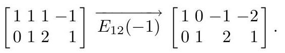
A=\left[\begin{array}{rrrr} 1 & 1 & 1 & -1 \\ 0 & 1 & 2 & 1 \end{array}\right]

So we want all \mathbf{x} with A\mathbf{x}=\mathbf{0}, i.e. the system \begin{aligned} x_{1}+x_{2}+x_{3}-x_{4} & =0 \\ x_{2}+2 x_{3}+x_{4} & =0 \end{aligned}

Step 1: Find the RREF of A.

Step 2: From RREF, pivots are in columns 1 and 2, so x_3 and x_4 are free; x_1 and x_2 are bound. Solve for the bound variables in terms of the free ones:

\begin{aligned} & x_{1}=x_{3}+2 x_{4} \\ & x_{2}=-2 x_{3}-x_{4} . \end{aligned}

Example: Finding the null space (continued)

From the previous slide we had x_1=x_3+2x_4, x_2=-2x_3-x_4 (free: x_3, x_4).

Step 3: Write the general solution \mathbf{x} as a linear combination of two vectors (one per free variable):

\left[\begin{array}{c} x_{1} \\ x_{2} \\ x_{3} \\ x_{4} \end{array}\right]=\left[\begin{array}{c} x_{3}+2 x_{4} \\ -2 x_{3}-x_{4} \\ x_{3} \\ x_{4} \end{array}\right]=x_{3}\left[\begin{array}{r} 1 \\ -2 \\ 1 \\ 0 \end{array}\right]+x_{4}\left[\begin{array}{r} 2 \\ -1 \\ 0 \\ 1 \end{array}\right] .

Step 4: Every solution is a linear combination of those two vectors, and they are linearly independent. So

\mathcal{N}(A)=\operatorname{span}\left\{\left[\begin{array}{r} 1 \\ -2 \\ 1 \\ 0 \end{array}\right],\left[\begin{array}{r} 2 \\ -1 \\ 0 \\ 1 \end{array}\right]\right\} \subseteq \mathbb{R}^{4}

and these two vectors form a basis for \mathcal{N}(A).

Using the null space to find a basis for the column space

Why does null space help?

The columns of A span \mathcal{C}(A), but they may be linearly dependent (redundant).
To get a basis, we want to drop columns that are linear combinations of the others.
The null space tells us those dependencies: every solution \mathbf{x} to A\mathbf{x}=\mathbf{0} gives x_1\mathbf{a}_1+\cdots+x_n\mathbf{a}_n=\mathbf{0}.
If x_j\neq 0, then \mathbf{a}_j is a combination of the other columns—so we can remove it from a spanning set.

Method: column space basis from null space

Find the null space (general solution to A\mathbf{x}=\mathbf{0}).
From that general solution, plug in simple choices (one free variable =1, rest =0) to get specific relations among the columns.
Each relation shows one column is redundant.
The columns that are not redundant (the pivot columns) form a basis for \mathcal{C}(A).

Example: Basis for column space from null space

Same matrix as before:

A=\left[\begin{array}{rrrr} 1 & 1 & 1 & -1 \\ 0 & 1 & 2 & 1 \end{array}\right]=\left[\mathbf{a}_{1}, \mathbf{a}_{2}, \mathbf{a}_{3}, \mathbf{a}_{4}\right]

We already found that the general solution to A\mathbf{x}=\mathbf{0} is \mathbf{x}=\left(x_{3}+2 x_{4},\,-2 x_{3}-x_{4},\, x_{3},\, x_{4}\right), so any solution satisfies \mathbf{0}=x_{1} \mathbf{a}_{1}+x_{2} \mathbf{a}_{2}+x_{3} \mathbf{a}_{3}+x_{4} \mathbf{a}_{4}.

Get dependency relations: Set one free variable to 1 and the others to 0.

x_3=1, x_4=0 \Rightarrow x_1=1, x_2=-2 \Rightarrow \mathbf{0}=\mathbf{a}_{1}-2\mathbf{a}_{2}+\mathbf{a}_{3}, so \mathbf{a}_{3}=\mathbf{a}_{1}+2\mathbf{a}_{2} (column 3 is redundant).
x_3=0, x_4=1 \Rightarrow x_1=2, x_2=-1 \Rightarrow \mathbf{0}=2\mathbf{a}_{1}-\mathbf{a}_{2}+\mathbf{a}_{4}, so \mathbf{a}_{4}=-2\mathbf{a}_{1}+\mathbf{a}_{2} (column 4 is redundant).

Example: Basis for column space (conclusion)

We had \mathbf{a}_3=\mathbf{a}_1+2\mathbf{a}_2 and \mathbf{a}_4=-2\mathbf{a}_1+\mathbf{a}_2, so columns 3 and 4 are redundant. Columns 1 and 2 (pivot columns) are linearly independent.

So a basis for \mathcal{C}(A) is \{\mathbf{a}_1,\mathbf{a}_2\}:

\mathcal{C}(A)=\operatorname{span}\left\{\mathbf{a}_{1}, \mathbf{a}_{2}\right\}=\operatorname{span}\left\{\left[\begin{array}{l}1 \\ 0\end{array}\right],\left[\begin{array}{l}1 \\ 1\end{array}\right]\right\}

Skills: Fundamental Subspaces

You should be able to:

Find a basis for the null space of a matrix.
Find a basis for the column space using the pivot-column / null-space method.
Determine if a matrix is invertible from its null space (\mathcal{N}(A)=\{\mathbf{0}\}).

Applications

Applications of null space and column space: finding equilibria, checking consistency, and describing solution sets.

Markov chain steady state (finding equilibrium)

Motivation:

In a Markov chain, a probability vector \mathbf{x}^{(k)} updates by \mathbf{x}^{(k+1)}=A\mathbf{x}^{(k)} for a fixed transition matrix A.
A steady state (equilibrium) is a vector \mathbf{x} that does not change under the update: \mathbf{x}=A\mathbf{x}.
We can find it using the null space of I-A.

Setup: Suppose the chain has a stable transition matrix A=\left[\begin{array}{ll}0.7 & 0.4 \\ 0.3 & 0.6\end{array}\right], so that \mathbf{x}^{(k+1)}=A \mathbf{x}^{(k)}. What is the steady-state vector \mathbf{x}? (The limit as k \rightarrow \infty of \mathbf{x}^{(k)}.)

Key step: At equilibrium, \mathbf{x}=A\mathbf{x}. Rearranging: \mathbf{x}-A\mathbf{x}=\mathbf{0} \quad\Rightarrow\quad (I-A)\mathbf{x}=\mathbf{0}.

So every steady-state vector must lie in \mathcal{N}(I-A).

There may be more than one vector in \mathcal{N}(I-A), but not all of them are valid probability distributions.

Our approach: find the null space; then pick the vector that is a valid probability distribution (nonnegative entries, sum 1).

Markov chain: finding \mathcal{N}(I-A)

Step 1: Compute I-A and row reduce:

I-A=\left[\begin{array}{rr} 0.3 & -0.4 \\ -0.3 & 0.4 \end{array}\right] \xrightarrow{\mathrm{RREF}}\left[\begin{array}{rr} 1 & -4/3 \\ 0 & 0 \end{array}\right].

Solution set: x_{1}=(4/3)x_{2}. So \mathcal{N}(I-A) is spanned by \mathbf{v}=(4/3, 1) (or equivalently (4,3)).

Markov chain: normalizing to a probability vector

\mathcal{N}(I-A) is spanned by (4/3, 1). Steady-state vectors must have nonnegative entries that sum to 1.

Step 2: The only such multiple with sum 1 is \frac{1}{(4/3)+1}(4/3,\,1) = \frac{3}{7}(4/3,\,1) = (4/7,\,3/7) \approx (0.571,\,0.429). So the unique steady-state (probability) vector is \mathbf{x}=(4/7,\,3/7).

Consistency and Column Space: Back to Linear Systems

When is A\mathbf{x}=\mathbf{b} consistent? That is, when does A\mathbf{x}=\mathbf{b} have a solution?

We can find the answer by looking at the column space of A.

The linear system A \mathbf{x}=\mathbf{b} of m equations in n unknowns is consistent if and only if \mathbf{b} \in \mathcal{C}(A).

In other words:

A\mathbf{x} is a linear combination of the columns of A (coefficients = entries of \mathbf{x}).
So A\mathbf{x}=\mathbf{b} has a solution exactly when \mathbf{b} is such a combination—i.e. \mathbf{b} \in \mathcal{C}(A).

Method: testing if a vector is in a spanning set

Goal: Decide whether \mathbf{b} \in \operatorname{span}\{\mathbf{v}_1,\ldots,\mathbf{v}_k\}.

Form A=[\mathbf{v}_1,\ldots,\mathbf{v}_k]. Then \mathbf{b} \in \mathcal{C}(A) iff A\mathbf{x}=\mathbf{b} is consistent.
Form the augmented matrix [A\mid\mathbf{b}] (or [A\mid\mathbf{b}_1\mid\mathbf{b}_2\mid\cdots] to test several vectors at once) and row reduce.
Decide consistency from the RREF:
- Pivot in an augmented column \Rightarrow a row [0\;\cdots\;0\mid 1] (i.e. 0=1) \Rightarrow inconsistent \Rightarrow that vector \notin \mathcal{C}(A).
- No pivot in that augmented column \Rightarrow consistent \Rightarrow that vector \in \mathcal{C}(A).

Example: which vector is in the span?

Let V=\operatorname{span}\{\mathbf{v}_1,\mathbf{v}_2,\mathbf{v}_3\} where
- \mathbf{v}_1=(1,1,3,3)
- \mathbf{v}_2=(0,2,2,4)
- \mathbf{v}_3=(1,0,2,1)
Which of the vectors is in V?
- \mathbf{u}=(2,1,5,4)
- \mathbf{w}=(1,0,0,0)

Form A=[\mathbf{v}_1,\mathbf{v}_2,\mathbf{v}_3] and [A\mid\mathbf{u}\mid\mathbf{w}], then row reduce:

[A \mid \mathbf{u} \mid \mathbf{w}]=\left[\begin{array}{lllll} 1 & 0 & 1 & 2 & 1 \\ 1 & 2 & 0 & 1 & 0 \\ 3 & 2 & 2 & 5 & 0 \\ 3 & 4 & 1 & 4 & 0 \end{array}\right] \quad \Longrightarrow \quad \mathrm{RREF}=\left[\begin{array}{rrrrr} 1 & 0 & 1 & 2 & 0 \\ 0 & 1 & -\frac{1}{2} & -\frac{1}{2} & 0 \\ 0 & 0 & 0 & 0 & 1 \\ 0 & 0 & 0 & 0 & 0 \end{array}\right]

Column 4 = \mathbf{u}, column 5 = \mathbf{w}. No pivot in column 4 \Rightarrow \mathbf{u} \in V; pivot in column 5 \Rightarrow \mathbf{w} \notin V.

One representation of \mathbf{u}:

From the general solution to A\mathbf{x}=\mathbf{u} (free variable c_3), we get

\mathbf{u}=(2-c_3)\mathbf{v}_1+\frac{1}{2}(c_3-1)\mathbf{v}_2+c_3\mathbf{v}_3.

Example: if c_3=0, then \mathbf{u}=2\mathbf{v}_1-\frac{1}{2}\mathbf{v}_2.

Form of general solution to a linear system

We know the solution set of A\mathbf{x}=\mathbf{0} is the null space (a subspace through the origin). For A\mathbf{x}=\mathbf{b} with \mathbf{b}\neq\mathbf{0}, the solution set is not a subspace—but once we find one particular solution, the rest of the solutions come from adding null-space vectors.

Suppose the system A \mathbf{x}=\mathbf{b} has a particular solution \mathbf{x}_{*}.
Then the general solution \mathbf{x} to this system can be described by the equation

\mathbf{x}=\mathbf{x}_{*}+\mathbf{z}

where \mathbf{z} runs over all elements of \mathcal{N}(A).

Form of general solution: geometry

So \mathbf{x}=\mathbf{x}_*+\mathbf{z} with \mathbf{z}\in\mathcal{N}(A).

Solution set is the set of all translates of the null space by the particular solution \mathbf{x}_*—a copy of the null space shifted away from the origin.

When the number of free variables is 1 or 2 (in 2D or 3D), the solution set is a point, a line, or a plane—not necessarily through the origin.

Example

Describe the solution set of the system \begin{array}{r} x+2 y=3 \\ x+y+z=3 . \end{array} (Three unknowns; one free variable.)

Parametric form: From x+2y=3 we get x=3-2y. Substituting into x+y+z=3 gives z=y. So the general solution is x=3-2t,\quad y=t,\quad z=t \quad (t \in \mathbb{R}). The solution set is a line in \mathbb{R}^3 (one free variable): not through the origin (particular solution (3,0,0) when t=0), in the direction of \mathbf{z}=(-2,1,1) \in \mathcal{N}(A).

Gas diffusion in a tube: matrices simplify physical systems

Motivation:

Diffusion (e.g., gas in a tube) spreads concentration from each point to its neighbors.
After discretizing space and time, the next value at site i depends on the current values at i-1, i, and i+1.
Stacking all sites into a vector turns the recurrence into a single matrix update: \mathbf{y}_{t+1}=(I+dM)\mathbf{y}_t.

Model: At each site i and time t, y_{i,\,t+1}=y_{i,\,t}+d\left(y_{i-1,\,t}-2y_{i,\,t}+y_{i+1,\,t}\right), with d=kD/h^2. Stack all sites into \mathbf{y}_t; then \mathbf{y}_{t+1}=(I+dM)\mathbf{y}_t for a simple banded matrix M.

Gas diffusion: inverse problem

Forward evolution: \mathbf{y}_{t+1}=(I+dM)\mathbf{y}_t. Given future \mathbf{y}_{t+1}, infer past \mathbf{y}_t:

Exact: \mathbf{y}_t=(I+dM)^{-1}\mathbf{y}_{t+1} (invert the matrix).
Approximate: \mathbf{y}_t\approx \mathbf{y}_{t+1}-dM\mathbf{y}_{t+1} (replace \mathbf{y}_t on the right by \mathbf{y}_{t+1} and solve once).

Why the approximation works:

For small d, Taylor series gives (I+dM)^{-1}=I-dM+O(d^2).
So \mathbf{y}_t=(I+dM)^{-1}\mathbf{y}_{t+1}\\approx (I-dM)\mathbf{y}_{t+1}, which matches the one-step approximation to first order in d.

Null Space algorithm

Given an m \times n matrix A.

Compute the reduced row echelon form R of A.
Use R to find the general solution to the homogeneous system A \mathbf{x}=0.
Write the general solution \mathbf{x}=\left(x_{1}, x_{2}, \ldots, x_{n}\right) to the homogeneous system in the form

\mathbf{x}=x_{i_{1}} \mathbf{w}_{1}+x_{i_{2}} \mathbf{w}_{2}+\cdots+x_{i_{n-r}} \mathbf{w}_{n-r}

where x_{i_{1}}, x_{i_{2}}, \ldots, x_{i_{n-r}} are the free variables.

List the vectors \mathbf{w}_{1}, \mathbf{w}_{2}, \ldots, \mathbf{w}_{n-r}. These form a basis of \mathcal{N}(A).

Skills: Applications

You should be able to:

Find steady-state vectors of Markov chains using the null space of I-A.
Determine if A\mathbf{x}=\mathbf{b} is consistent using column space (\mathbf{b}\in\mathcal{C}(A)).
Describe solution-set geometry (point, line, plane) using null space and particular solutions.