import plotly.graph_objects as go
import numpy as np

# Column space basis and example vectors (all in C(A))
a1 = np.array([1, 1, 2])
a2 = np.array([1, 2, 1])
example_vectors = [
    np.array([1, 1, 2]),
    np.array([1, 2, 1]),
    np.array([2, 3, 3]),
    np.array([3, 3, 6]),
]

# Create figure (plane not shown, only vectors)
fig = go.Figure()

# Colors for each vector for contrast
colors = ['crimson', 'darkorange', 'seagreen', 'royalblue']
for v, c in zip(example_vectors, colors):
    fig.add_trace(go.Scatter3d(
        x=[0, v[0]], y=[0, v[1]], z=[0, v[2]],
        mode='lines+markers',
        line=dict(width=7, color=c),
        marker=dict(size=7, color=c),
        showlegend=False  # Hide legend
    ))

fig.update_layout(
    title=dict(text="Column space and example vectors", x=0.5),
    scene=dict(
        xaxis_title="x",
        yaxis_title="y",
        zaxis_title="z",
        aspectmode='data',
        camera=dict(eye=dict(x=1.4, y=1.4, z=1.1))
    ),
    margin=dict(l=0, r=0, b=0, t=30),
    height=420,
    template='plotly_white',
    showlegend=False  # Hide legend
)
fig.show()Ch4 Lecture 1
Geometrical View of Column Space
Why column space matters
- Consistency of \(A\mathbf{x}=\mathbf{b}\): solvable exactly when \(\mathbf{b} \in \mathcal{C}(A)\) (the “reachable” set).
- Least squares: Later today: when \(\mathbf{b} \notin \mathcal{C}(A)\), we find the closest point in \(\mathcal{C}(A)\) to \(\mathbf{b}\) (projection onto the column space).
- Seeing \(\mathcal{C}(A)\) as a line or plane makes this concrete.
Example: a rank-1 matrix
\[ A = \begin{bmatrix} 1 & 2 & 0 \\ 1 & 2 & 0 \\ 0 & 0 & 0 \end{bmatrix} \]
Columns are \(\mathbf{a}_1 = (1,1,0)\), \(\mathbf{a}_2 = 2\mathbf{a}_1\), \(\mathbf{a}_3 = \mathbf{0}\).
. . .
The only vectors that we can form by taking linear combinations of the columns of \(A\) are multiples of \(\begin{bmatrix} 1 \\ 1 \\ 0 \end{bmatrix}\).
. . .
A basis for the column space is just this single vector: \(\left\lbrace \begin{bmatrix} 1 \\ 1 \\ 0 \end{bmatrix} \right\rbrace\).
. . .
Because there is only one vector in the basis, the matrix has rank 1.
Visualizing the column space of our rank-1 matrix
Here are some vectors that are in the column space of \(A\):
\[ \begin{bmatrix} 1 \\ 1 \\ 0 \end{bmatrix}, \begin{bmatrix} 2 \\ 2 \\ 0 \end{bmatrix}, \begin{bmatrix} 3 \\ 3 \\ 0 \end{bmatrix}, \begin{bmatrix} 4 \\ 4 \\ 0 \end{bmatrix}, \begin{bmatrix} 5 \\ 5 \\ 0 \end{bmatrix}, \begin{bmatrix} -1 \\ -1 \\ 0 \end{bmatrix}, \begin{bmatrix} -2 \\ -2 \\ 0 \end{bmatrix} \]
. . .
If we draw these vectors in \(\mathbb{R}^3\), we see that they all lie on the same line. This line is the column space of \(A\).
(draw it)
Remember, the column space tells us which vectors \(\mathbf{b}\) can be written as \(A\mathbf{x}\) for some \(\mathbf{x}\).
. . .
So if a vector \(\mathbf{b}\) is not on this line, we know that there is no solution to \(A\mathbf{x}=\mathbf{b}\).
. . .
(draw a b slightly off the line, and one very far off the line)
Example: a rank-2 matrix
\[ A = \begin{bmatrix} 1 & 1 & 2 \\ 1 & 2 & 3 \\ 2 & 1 & 3 \end{bmatrix} \]
. . .
The first two columns are independent, but the third is a linear combination of the first two.
. . .
We can make a basis for the column space by taking the first two columns: \(\left\lbrace \begin{bmatrix} 1 \\ 1 \\ 2 \end{bmatrix}, \begin{bmatrix} 1 \\ 2 \\ 1 \end{bmatrix} \right\rbrace\).
\[ \mathcal{C}(A) = \mathrm{span}\left\lbrace \begin{bmatrix} 1 \\ 1 \\ 2 \end{bmatrix}, \begin{bmatrix} 1 \\ 2 \\ 1 \end{bmatrix} \right\rbrace \]
Here are some vectors that are in the column space of \(A\):
\[ \begin{bmatrix} 1 \\ 1 \\ 2 \end{bmatrix} = 1 \cdot \mathbf{a}_1 + 0 \cdot \mathbf{a}_2, \qquad \begin{bmatrix} 1 \\ 2 \\ 1 \end{bmatrix} = 0 \cdot \mathbf{a}_1 + 1 \cdot \mathbf{a}_2, \]
\[ \begin{bmatrix} 2 \\ 3 \\ 3 \end{bmatrix} = 1 \cdot \mathbf{a}_1 + 1 \cdot \mathbf{a}_2, \qquad \begin{bmatrix} 3 \\ 3 \\ 6 \end{bmatrix} = 3 \cdot \mathbf{a}_1 + 0 \cdot \mathbf{a}_2 \]
Visualizing the column space of our rank-2 matrix
import plotly.graph_objects as go
import numpy as np

# Column space basis and example vectors (all in C(A))
a1 = np.array([1, 1, 2])
a2 = np.array([1, 2, 1])
example_vectors = [
    np.array([1, 1, 2]),
    np.array([1, 2, 1]),
    np.array([2, 3, 3]),
    np.array([3, 3, 6]),
]

# Create figure
fig = go.Figure()

# Add the filled plane span{a1, a2} through origin (large extent)
s = np.linspace(-3.75, 3.75, 24)
t = np.linspace(-3.75, 3.75, 24)
S, T = np.meshgrid(s, t)
X = S * a1[0] + T * a2[0]
Y = S * a1[1] + T * a2[1]
Z = S * a1[2] + T * a2[2]
fig.add_trace(go.Surface(
    x=X, y=Y, z=Z,
    colorscale=[[0, 'lightblue'], [1, 'lightblue']],
    opacity=0.45,
    showscale=False,
    name="Plane"
))

# Colors for each vector for contrast
colors = ['crimson', 'darkorange', 'seagreen', 'royalblue']
for v, c in zip(example_vectors, colors):
    fig.add_trace(go.Scatter3d(
        x=[0, v[0]], y=[0, v[1]], z=[0, v[2]],
        mode='lines+markers',
        line=dict(width=7, color=c),
        marker=dict(size=7, color=c),
        showlegend=False  # Hide legend
    ))

fig.update_layout(
    title=dict(text="Column space (plane filled) and example vectors", x=0.5),
    scene=dict(
        xaxis_title="x",
        yaxis_title="y",
        zaxis_title="z",
        aspectmode='data',
        camera=dict(eye=dict(x=0.9, y=0.9, z=0.7))
    ),
    margin=dict(l=0, r=0, b=0, t=30),
    height=420,
    template='plotly_white',
    showlegend=False
)
fig.show()
General form of the column space in \(\mathbb{R}^3\)
In \(\mathbb{R}^3\), the dimension of \(\mathcal{C}(A)\) equals the rank \(r\) of \(A\):
- Rank 1: \(\mathcal{C}(A)\) is a line (all columns are multiples of one vector).
- Rank 2: \(\mathcal{C}(A)\) is a plane (span of two independent columns).
- Rank 3: \(\mathcal{C}(A)\) is all of \(\mathbb{R}^3\).
General form of the column space in \(\mathbb{R}^n\)
In \(\mathbb{R}^n\), the dimension of \(\mathcal{C}(A)\) equals the rank \(r\) of \(A\):
- Rank 1: \(\mathcal{C}(A)\) is a line (all columns are multiples of one vector).
- Rank 2: \(\mathcal{C}(A)\) is a plane (span of two independent columns).
- Rank n-1: \(\mathcal{C}(A)\) is a hyperplane (span of n-1 independent columns in \(\mathbb{R}^n\)).
Input and output spaces
The pictures we have drawn of the column space represent the possible outputs \(\mathbf{b}\) from the linear system \(A\mathbf{x}=\mathbf{b}\).
. . .
In our example, all potential outputs \(\mathbf{b}\) live in \(\mathbb{R}^3\), but the only ones that are actually reachable are those that are on a line or a plane within \(\mathbb{R}^3\). So the column space of \(A\) is a special subspace of the output space.
. . .
Formally, we call the output space the codomain of \(A\), and the column space of \(A\) is a subspace of the codomain.
. . .
But there’s another space that’s important: the space of all the possible inputs \(\mathbf{x}\) that can be fed into \(A\). We call this the domain of \(A\).
In our examples so far, because the vectors \(\mathbf{x}\) are all in \(\mathbb{R}^3\), the domain is also \(\mathbb{R}^3\).
Domain and codomain for a rectangular matrix
Let’s consider a simple 2x3 matrix:
\[ F = \begin{bmatrix} 1 & 2 & 0 \\ 1 & 2 & 0 \end{bmatrix} \]
. . .
For the system \(F\mathbf{x}=\mathbf{b}\), the possible inputs \(\mathbf{x}\) are all in \(\mathbb{R}^3\), and the possible outputs \(\mathbf{b}\) are all in \(\mathbb{R}^2\).
. . .
For example, if we take \(\mathbf{x} = \begin{bmatrix} 1 \\ 2 \\ 3 \end{bmatrix}\), then \[ F\mathbf{x} = \begin{bmatrix} 1 & 2 & 0 \\ 1 & 2 & 0 \end{bmatrix} \begin{bmatrix} 1 \\ 2 \\ 3 \end{bmatrix} = \begin{bmatrix} 5 \\ 5 \end{bmatrix} = \mathbf{b} \]
So \(\mathbf{x}=\begin{bmatrix} 1 \\ 2 \\ 3 \end{bmatrix}\) is in the domain of \(F\), and \(\mathbf{b}=\begin{bmatrix} 5 \\ 5 \end{bmatrix}\) is in the codomain of \(F\).
Column space and null space are special subspaces
We know that \(\mathbf{b}=\begin{bmatrix} 5 \\ 5 \end{bmatrix}\) is in the column space of \(F\) because we constructed it from multiplying \(F\) by \(\mathbf{x}\).
. . .
There are other vectors, such as \(\begin{bmatrix} 1 \\ -1 \end{bmatrix}\), that are in the codomain of \(F\) but not in its column space.
. . .
The column space is a subspace of the codomain, and it tells us something about the matrix \(F\).
Is there a similar special subset of the vectors in the domain that tells us something about the matrix \(F\)? There is!
. . .
Yes, it’s the null space of \(F\). The null space of \(F\) is the set of all vectors \(\mathbf{x}\) such that \(F\mathbf{x}=\mathbf{0}\).
. . .
For example, the vector \(\begin{bmatrix} 1 \\ -1 \\ 0 \end{bmatrix}\) is in the null space of \(F\) because \[ F\begin{bmatrix} 1 \\ -1 \\ 0 \end{bmatrix} = \begin{bmatrix} 1 & 2 & 0 \\ 1 & 2 & 0 \end{bmatrix} \begin{bmatrix} 1 \\ -1 \\ 0 \end{bmatrix} = \begin{bmatrix} 1 \cdot 1 + 2 \cdot (-1) + 0 \cdot 0 \\ 1 \cdot 1 + 2 \cdot (-1) + 0 \cdot 0 \end{bmatrix} = \begin{bmatrix} 0 \\ 0 \end{bmatrix} = \mathbf{0} \]
Visualizing the null space
If we know a basis for the null space, we can visualize it in the domain.
. . .
We haven’t learned how to find these yet, but for our example matrix \(F=\begin{bmatrix} 1 & 2 & 0 \\ 1 & 2 & 0 \end{bmatrix}\), I’ll just tell you that the basis for the null space is \(\left\lbrace \begin{bmatrix} -2 \\ 1 \\ 0 \end{bmatrix}, \begin{bmatrix} 0 \\ 0 \\ 1 \end{bmatrix} \right\rbrace\).
. . .
So the null space will form a plane in \(\mathbb{R}^3\).
Visualizing both the column space and the null space
But because the null space is a subspace of the input space (the domain) and the column space is a subspace of the output space (the codomain), we can’t visualize them together in the same picture.
So we’ll visualize them separately.
The column space \(\mathcal{C}(F)\) is all vectors in \(\mathbb{R}^2\) that are multiples of \(\begin{bmatrix} 1 \\ 1 \end{bmatrix}\).
The null space \(\mathcal{N}(F)\) is that spanned by the vectors \(\begin{bmatrix} -2 \\ 1 \\ 0 \end{bmatrix}\) and \(\begin{bmatrix} 0 \\ 0 \\ 1 \end{bmatrix}\).
import numpy as np
import matplotlib.pyplot as plt

fig = plt.figure(figsize=(12, 5))

# First subplot: column space in 2D (a line in R^2)
ax1 = fig.add_subplot(1, 2, 1)
# Line through origin along [1, 1]
t = np.linspace(-3, 3, 100)
line = np.vstack((t, t))  # [t, t] for t in R

ax1.plot(line[0], line[1], color='royalblue', lw=2, label='Column space')
ax1.scatter([0], [0], color='black')  # origin
ax1.set_xlabel("$b_1$")
ax1.set_ylabel("$b_2$")
ax1.set_title(r"Column space in $\mathbb{R}^2$")
ax1.grid(True)
ax1.set_aspect('equal')
ax1.legend()

# Second subplot: null space in 3D (a plane in R^3)
from mpl_toolkits.mplot3d import Axes3D  # noqa: F401

ax2 = fig.add_subplot(1, 2, 2, projection='3d')

# The null space plane: spanned by [-2, 1, 0] and [0, 0, 1]
s = np.linspace(-2, 2, 20)
t = np.linspace(-2, 2, 20)
S, T = np.meshgrid(s, t)
X = -2*S
Y = S
Z = T
# Plane points: for each (s, t): s * [-2,1,0] + t * [0,0,1]
ax2.plot_surface(X, Y, Z, alpha=0.4, color='tomato', rstride=1, cstride=1, edgecolor='none')

# Draw the two basis vectors of the plane
ax2.quiver(0, 0, 0, -2, 1, 0, color='maroon', length=2.2, normalize=True, linewidth=2)
ax2.quiver(0, 0, 0, 0, 0, 1, color='darkred', length=2.2, normalize=True, linewidth=2)

ax2.set_xlabel("$x_1$")
ax2.set_ylabel("$x_2$")
ax2.set_zlabel("$x_3$")
ax2.set_title("Null space in $\mathbb{R}^3$")
ax2.view_init(elev=18, azim=121)

plt.tight_layout()
plt.show()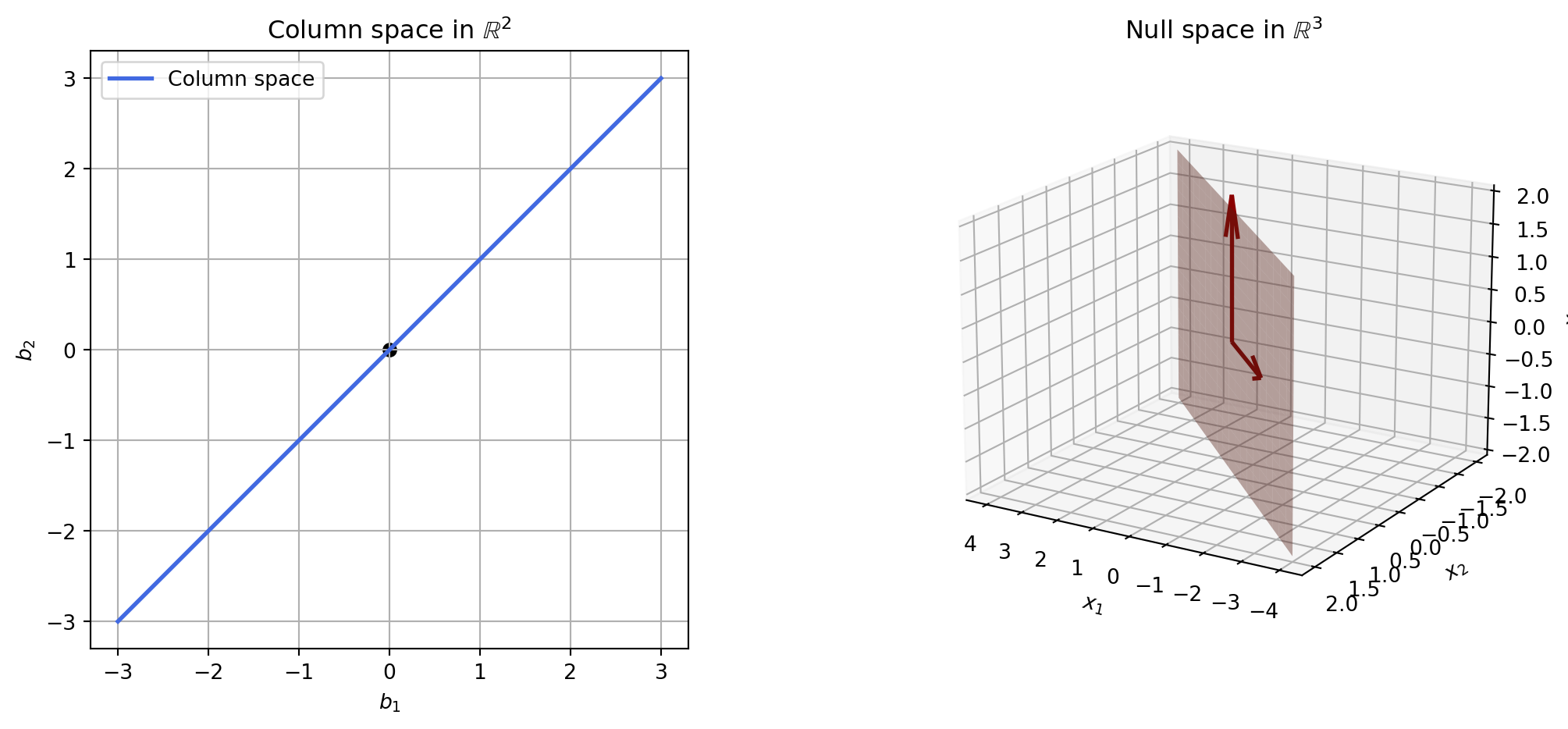
Row space and left null space
The row space of a matrix \(A\) is the subspace of \(\mathbb{R}^m\) spanned by the rows of \(A\). It is also the column space of \(A^T\).
The left null space of a matrix \(A\) is just the null space of \(A^T\).
Skills: Fundamental Subspaces (Pictures)
- Interpret \(\mathcal{C}(A)\) geometrically (line, plane, or hyperplane) from the rank of \(A\).
- Distinguish between the domain (where \(\mathbf{x}\) lives) and codomain (where \(A\mathbf{x}\) lives) for a matrix.
- Identify the column space as a subspace of the codomain; the null space as a subspace of the domain.
- Given a basis for \(\mathcal{N}(A)\), describe its shape (line, plane, etc.) in the input space.
Planes, Hyperplanes, and Projections
The plane through the origin
Because the column space is so often a plane, let’s build our intuition about planes.
A plane through the origin is the set of all vectors \(\vec x\) such that \(\vec a \cdot \vec x = 0\), where the nonzero vector \(\vec a\) is a normal vector to the plane (we often take \(\vec a\) of unit length).
. . .
Finding the normal vector when we know two vectors in the plane
For \(\mathbb{R}^3\), we can find the normal vector by taking the cross product of two vectors in the plane.
Let \(\mathbf{i}, \mathbf{j}\), and \(\mathbf{k}\) represent the standard basis \(\mathbf{e}_{1}, \mathbf{e}_{2}, \mathbf{e}_{3}\).
\[ \mathbf{u} \times \mathbf{v}=\left(u_{2} v_{3}-u_{3} v_{2}\right) \mathbf{i}+\left(u_{3} v_{1}-u_{1} v_{3}\right) \mathbf{j}+\left(u_{1} v_{2}-u_{2} v_{1}\right) \mathbf{k}=\left|\begin{array}{ccc} \mathbf{i} & \mathbf{j} & \mathbf{k} \\ u_{1} & u_{2} & u_{3} \\ v_{1} & v_{2} & v_{3} \end{array}\right| \]
. . .
The cross product is orthogonal to both \(\mathbf{u}\) and \(\mathbf{v}\): \(\mathbf{u} \cdot (\mathbf{u} \times \mathbf{v})=0\) and \(\mathbf{v} \cdot (\mathbf{u} \times \mathbf{v})=0\).
. . .
We can use the cross product to find the normal vector to the plane by taking the cross product of two vectors in the plane.
Finding the normal vector from the equation of the plane
If the plane is specified by \(ax + by + cz = d\), then a normal vector is \(\vec a = (a, b, c)\).
. . .
Check (optional verification):
- Find three points on the plane: e.g. \((0, 0, d/c)\), \((0, d/b, 0)\), \((d/a, 0, 0)\) (when \(a,b,c \neq 0\)).
- Form two displacement vectors in the plane, e.g. \(\vec u = (0, d/b, -d/c)\) and \(\vec v = (d/a, 0, -d/c)\).
. . .
Verifying the normal from \(ax+by+cz=d\)
Take the cross product \(\vec u \times \vec v\):
\[ \begin{aligned} \vec u \times \vec v &= \left|\begin{array}{ccc} \mathbf{i} & \mathbf{j} & \mathbf{k} \\ 0 & d/b & -d/c \\ d/a & 0 & -d/c \end{array}\right| \\ &= -\frac{d^2}{bc} \mathbf{i} + \frac{d^2}{ac} \mathbf{j} - \frac{d^2}{ab} \mathbf{k} = -\frac{d^2}{abc} \left( a \mathbf{i} - b \mathbf{j} + c \mathbf{k} \right) \end{aligned} \]
This is parallel to \(\vec{a} = (a, b, c)\).
. . .
Distances from the plane
The distance from a point \(\vec x\) to the plane \(\vec a \cdot \vec x = 0\) is the scalar projection of \(\vec x\) onto the normal:
- If \(\vec a\) is unit length: distance \(= |\vec a \cdot \vec x|\).
- If not: distance \(= |\vec a \cdot \vec x| / \|\vec a\|\).
. . .
Closest point on the plane (through the origin)
The displacement from \(\vec x\) to the closest point on the plane has length \(|\vec a \cdot \vec x|/\|\vec a\|\) and direction along \(\vec a\).
. . .
Projection onto the plane (through the origin)
The closest point on the plane to \(\vec x\) is \(\vec x - \vec a (\vec x \cdot \vec a)/\|\vec a\|^2\) — i.e., \(\vec x\) minus the projection of \(\vec x\) onto \(\vec a\).
A plane not at the origin
A plane displaced from the origin can be described by a normal \(\vec a\) and a scalar \(q\): the plane is displaced by \(q \vec a\) from the origin.
. . .
Equation of the displaced plane
Points \(\vec x\) on the plane satisfy \(\vec a \cdot \vec x = q\) (with \(\vec a\) unit length, \(q\) is the signed distance of the plane from the origin).
. . .
Hyperplane
A hyperplane in \(\mathbb{R}^{n}\) is the set of all \(\mathbf{x} \in \mathbb{R}^{n}\) such that \(\mathbf{a} \cdot \mathbf{x}=b\), where the nonzero vector \(\mathbf{a} \in \mathbb{R}^{n}\) and scalar \(b\) are given.
. . .
Let \(H\) be the hyperplane in \(\mathbb{R}^{n}\) defined by \(\mathbf{a} \cdot \mathbf{x}=b\) and let \(\mathbf{x}_{*} \in H\). Then
\(\mathbf{a}^{\perp}=\{\mathbf{y} \in \mathbb{R}^{n} \mid \mathbf{a} \cdot \mathbf{y}=0\}\) is a subspace of \(\mathbb{R}^{n}\) of dimension \(n-1\).
\(H=\mathbf{x}_{*}+\mathbf{a}^{\perp}=\{\mathbf{x}_{*}+\mathbf{y} \mid \mathbf{y} \in \mathbf{a}^{\perp}\}\).
. . .
Example: plane through three points
Find an equation that defines the plane containing the three (noncollinear) points \(P, Q\), and \(R\) with coordinates \((1,0,2)\), \((2,1,0)\), and \((3,1,1)\), respectively.
. . .
\[ \begin{aligned} \overrightarrow{P Q}&=(2,1,0)-(1,0,2)=(1,1,-2) \\ \overrightarrow{P R}&=(3,1,1)-(1,0,2)=(2,1,-1) \end{aligned} \]
. . .
\[ \mathbf{u} \times \mathbf{v}=\left|\begin{array}{ccc} \mathbf{i} & \mathbf{j} & \mathbf{k} \\ 1 & 1 & -2 \\ 2 & 1 & -1 \end{array}\right|=\mathbf{i}-3 \mathbf{j}-\mathbf{k} \]
. . .
The normal vector is \(\mathbf{a}=(1,-3,-1)\).
. . .
The equation of the plane is \(\mathbf{a} \cdot \mathbf{x}=b\). Using \(P\): \(b=\mathbf{a} \cdot \mathbf{P}=(1,-3,-1) \cdot (1,0,2)=1+0-2=-1\).
. . .
So the plane is \(x - 3y - z = -1\).
Projections to the displaced plane
The closest point on the hyperplane \(\vec a \cdot \vec x = q\) to a point \(\vec x\) is \(\vec x - \vec a (\vec a \cdot \vec x - q)\) (for unit \(\vec a\)).
. . .
Summary: planes and projections
- Plane through the origin: \(\vec a \cdot \vec x = 0\).
- Plane displaced: \(\vec a \cdot \vec x = q\).
- Scalar projection of \(\vec x\) onto \(\vec a\): \(\vec a \cdot \vec x / \|\vec a\|\).
- Vector projection of \(\vec x\) onto \(\vec a\): \(\frac{\vec a}{\|\vec a\|} \frac{\vec a \cdot \vec x}{\|\vec a\|}\).
- Projection of \(\vec x\) onto the plane \(\vec a \cdot \vec x = q\): \(\vec x - \vec a (\vec a \cdot \vec x - q)\).
. . .
Projection formula for vectors
Let \(\mathbf{u}\) and \(\mathbf{v}\) be vectors, \(\mathbf{v} \neq \mathbf{0}\).
\[ \mathbf{p}=\frac{\mathbf{v} \cdot \mathbf{u}}{\mathbf{v} \cdot \mathbf{v}} \mathbf{v} \quad \text{and} \quad \mathbf{q}=\mathbf{u}-\mathbf{p} \]
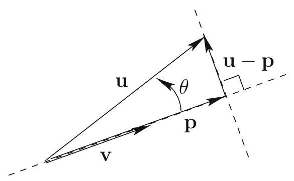
. . .
Then \(\mathbf{p}\) is parallel to \(\mathbf{v}\), \(\mathbf{q}\) is orthogonal to \(\mathbf{v}\), and \(\mathbf{u}=\mathbf{p}+\mathbf{q}\).
. . .
We write \(\operatorname{proj}_{\mathbf{v}} \mathbf{u}=\frac{\mathbf{v} \cdot \mathbf{u}}{\mathbf{v} \cdot \mathbf{v}} \mathbf{v}\) and \(\operatorname{orth}_{\mathbf{v}} \mathbf{u}=\mathbf{u}-\operatorname{proj}_{\mathbf{v}} \mathbf{u}\).
. . .
Skills: Planes and Projections
- Write the equation of a plane (through the origin or displaced) using a normal vector.
- Find a normal to a plane from two vectors in the plane (cross product in \(\mathbb{R}^3\)) or from \(ax+by+cz=d\).
- Compute distance from a point to a plane and the projection of a point onto a plane.
- Use \(\operatorname{proj}_{\mathbf{v}} \mathbf{u}\) and \(\operatorname{orth}_{\mathbf{v}} \mathbf{u}\).
. . .
Least Squares
Least squares: project \(\mathbf{b}\) onto \(\mathcal{C}(A)\)
When \(A\mathbf{x}=\mathbf{b}\) is inconsistent, \(\mathbf{b}\) is not in the column space. Least squares finds \(\widehat{\mathbf{x}}\) so that \(A\widehat{\mathbf{x}}\) is the closest point in \(\mathcal{C}(A)\) to \(\mathbf{b}\)—i.e., the projection of \(\mathbf{b}\) onto the plane \(\mathcal{C}(A)\). The residual \(\mathbf{b} - A\widehat{\mathbf{x}}\) is perpendicular to \(\mathcal{C}(A)\).
. . .
import plotly.graph_objects as go
import numpy as np

# C(A) = xy-plane; take b = (0, 0, 1) so projection = (0,0,0), residual = (0,0,1)
s = np.linspace(-1.2, 1.2, 15)
t = np.linspace(-1.2, 1.2, 15)
S, T = np.meshgrid(s, t)
fig = go.Figure()
fig.add_trace(go.Surface(x=S, y=T, z=np.zeros_like(S), colorscale=[[0,'lightblue'],[1,'lightblue']], opacity=0.6, showscale=False, name=r"$\mathcal{C}(A)$"))
# b
fig.add_trace(go.Scatter3d(x=[0], y=[0], z=[1], mode='markers+text', text=[r"$\mathbf{b}$"], textposition='top center',
                           marker=dict(size=10, color='red', symbol='diamond'), name=r"$\mathbf{b}$"))
# projection = origin
fig.add_trace(go.Scatter3d(x=[0], y=[0], z=[0], mode='markers+text', text=[r"$\widehat{\mathbf{b}}$"], textposition='bottom center',
                           marker=dict(size=10, color='green', symbol='square'), name=r"$\widehat{\mathbf{b}}$"))
# residual from (0,0,0) to (0,0,1)
fig.add_trace(go.Scatter3d(x=[0, 0], y=[0, 0], z=[0, 1], mode='lines', line=dict(color='purple', width=6, dash='dash'), name="residual"))
fig.update_layout(scene=dict(xaxis_title="x", yaxis_title="y", zaxis_title="z", aspectmode='data',
                              camera=dict(eye=dict(x=1.3, y=1.3, z=1.0))),
                  title=dict(text=r"Projection of b onto C(A): residual ⟂ plane", x=0.5),
                  margin=dict(l=0, r=0, b=0, t=50), template='plotly_white', height=420)
fig.show()
. . .
Motivation: fitting a line to data
- We have data \((x_i, y_i)\) and want a line \(y \approx mx\) (or \(y \approx mx + b\)).
- The system \(\mathbf{y} = m \mathbf{x}\) is usually inconsistent.
- We choose \(m\) so that the residuals \(\mathbf{y} - m\mathbf{x}\) are as small as possible in a precise sense.
. . .
From \(\mathbb{R}^2\) to \(\mathbb{R}^n\)
- Think of the predictor values as a vector \(\mathbf{x} \in \mathbb{R}^n\) and the response values as \(\mathbf{y} \in \mathbb{R}^n\).
- A perfect linear relation means \(\mathbf{y} = m \mathbf{x}\) for some scalar \(m\).
. . .
Imperfect data
When data are not on a line, \(\mathbf{y} - m\mathbf{x} \neq \mathbf{0}\). The vector \(\mathbf{y} - m\mathbf{x}\) is the residual vector; we minimize \(\|\mathbf{y} - m\mathbf{x}\|^2\).
. . .
Best choice of \(m\)
The best \(m\) minimizes \(\|\mathbf{y} - m\mathbf{x}\|^2\). Geometrically, that happens when the residual \(\mathbf{y} - m\mathbf{x}\) is orthogonal to \(\mathbf{x}\).
. . .
Normal equation: one predictor
\(m \mathbf{x} - \mathbf{y}\) should be orthogonal to \(\mathbf{x}\), so \(\mathbf{x} \cdot (m \mathbf{x} - \mathbf{y}) = 0\).
\[ \begin{aligned} m \mathbf{x} \cdot \mathbf{x} - \mathbf{x} \cdot \mathbf{y} &= 0 \\ m \,\mathbf{x} \cdot \mathbf{x} &= \mathbf{x} \cdot \mathbf{y} \end{aligned} \]
. . .
Matching to general matrix notation: In the general problem \(\mathbf{A}\mathbf{x} = \mathbf{b}\), the pieces correspond to:
| Regression | General | Role |
|---|---|---|
| predictor \(\mathbf{x}\) | \(\mathbf{A}\) (known matrix/vector) | the data we observe |
| slope \(m\) | \(\mathbf{x}\) (unknown) | the parameter to solve for |
| response \(\mathbf{y}\) | \(\mathbf{b}\) (known vector) | the target we want to match |
. . .
Now translate the orthogonality condition step by step:
| Regression (dot products) | General (matrix notation) |
|---|---|
| \(\mathbf{x} \cdot (m\mathbf{x} - \mathbf{y}) = 0\) | \(\mathbf{A}^T(\mathbf{A}\mathbf{x} - \mathbf{b}) = \mathbf{0}\) |
| \(m\,\mathbf{x} \cdot \mathbf{x} = \mathbf{x} \cdot \mathbf{y}\) | \(\mathbf{A}^T \mathbf{A}\,\mathbf{x} = \mathbf{A}^T \mathbf{b}\) |
The \(\mathbf{A}^T\) comes from “dot with the data”: in the regression version we dot both sides with the predictor \(\mathbf{x}\); in matrix notation, that becomes multiplying on the left by \(\mathbf{A}^T\).
. . .
\[ \mathbf{A}^T \mathbf{A}\, \mathbf{x} = \mathbf{A}^T \mathbf{b} \]
These are the normal equations.
. . .
Single predictor: scalar case
When there is one predictor and one response, \(\mathbf{x}\) (the unknown) is a scalar. Write the predictor vector as \(\mathbf{a}\) and the response vector as \(\mathbf{b}\). Then:
\[ \mathbf{a}^T \mathbf{a}\, x = \mathbf{a}^T \mathbf{b} \quad \Rightarrow \quad x = \frac{\mathbf{a} \cdot \mathbf{b}}{\mathbf{a} \cdot \mathbf{a}} \]
This is the slope of the least-squares line (through the origin).
. . .
Example: scale calibration
You have a scale that measures in unknown units. You have items of known weight approximately 2, 5, and 7 pounds. You measure the scale output and get \(0.7\), \(2.4\), and \(3.2\). What is the conversion factor from the scale’s units to pounds?
. . .
Set \(\mathbf{a}= [2,\, 5,\, 7]^T\) and \(\mathbf{b}= [0.7,\, 2.4,\, 3.2]^T\). We want \(x\) such that \(\mathbf{a} \cdot x = \mathbf{b}\) (componentwise); the system is inconsistent, so we use least squares.
. . .
\[ \mathbf{a}^T \mathbf{a}\, x = \mathbf{a}^T \mathbf{b} \quad \Rightarrow \quad x = \frac{2(0.7) + 5(2.4) + 7(3.2)}{2^2 + 5^2 + 7^2} \approx 0.459 \]
So to convert from scale units to pounds, multiply by \(\approx 0.459\) (i.e., scale reading \(\times 0.459 \approx\) pounds).
. . .
(Book may use the opposite convention: conversion from pounds to scale units.)
. . .
Skills: Least Squares
- Set up the least-squares problem when \(\mathbf{A}\mathbf{x}=\mathbf{b}\) is inconsistent: minimize \(\|\mathbf{A}\mathbf{x}-\mathbf{b}\|^2\).
- Write and use the normal equations \(\mathbf{A}^T \mathbf{A} \mathbf{x} = \mathbf{A}^T \mathbf{b}\).
- For a single predictor (vector \(\mathbf{a}\), response \(\mathbf{b}\)), compute the best-fit scalar \(x = (\mathbf{a} \cdot \mathbf{b})/(\mathbf{a} \cdot \mathbf{a})\).