# Do imports
import networkx as nx
import matplotlib.pyplot as plt
import scipy
import numpy as npMCMC Pagerank
# Create a directed graph
G = nx.DiGraph()

# Add nodes
G.add_nodes_from([1, 2, 3, 4, 5, 6])

# Add vertices
edges = [(1, 2), (1, 3), (3, 2), (3, 1), (3, 4), (5, 6), (6, 5),(3,2),(2,4),(4,1)]
G.add_edges_from(edges)

# Draw the graph
nx.draw_circular(G, with_labels=True)
plt.show()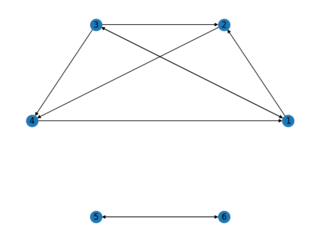
# Since the graph G is a DiGraph (Directed Graph), we can use the adjacency_matrix method from networkx to get the adjacency matrix
# Then, we normalize each row to sum to 1 to get the transition matrix

# Get the adjacency matrix (returns a scipy sparse matrix)
adj_matrix = nx.adjacency_matrix(G)

# Convert to a dense numpy array
adj_matrix = adj_matrix.toarray()

# Calculate the sum of each row
row_sums = adj_matrix.sum(axis=1)

# Normalize the matrix (this is the transition matrix)
transition_matrix = adj_matrix / row_sums[:, np.newaxis]
print(transition_matrix.T)
[[0. 0. 0.33333333 1. 0. 0. ]
[0.5 0. 0.33333333 0. 0. 0. ]
[0.5 0. 0. 0. 0. 0. ]
[0. 1. 0.33333333 0. 0. 0. ]
[0. 0. 0. 0. 0. 1. ]
[0. 0. 0. 0. 1. 0. ]]If not doing pagerank: Initializing a random stochastic matrix
import numpy as np

# Create a 6x6 matrix with random values
matrix = np.random.rand(6, 6)

# Normalize the matrix to make it a stochastic matrix
stochastic_matrix = matrix / matrix.sum(axis=1, keepdims=True)

# Square the matrix to increase the difference between values
matrix_squared = np.square(stochastic_matrix)

# Normalize the squared matrix to make it a stochastic matrix
stochastic_matrix_squared = matrix_squared / matrix_squared.sum(axis=1, keepdims=True)
Finding the stationary state of the matrix
# Normalize the teleportation matrix
teleportation = np.ones(np.shape(transition_matrix))
row_sums = teleportation.sum(axis=1)
teleportation = teleportation / row_sums[:, np.newaxis]

alpha = .15

transition_matrix_combined = (1-alpha)*transition_matrix + alpha*teleportation
# Use the transition matrix from the pagerank
stochastic_matrix = transition_matrix_combined

# Compute the eigenvalues and right eigenvectors
eigenvalues, eigenvectors = np.linalg.eig(np.transpose(stochastic_matrix))

# Find the index of the eigenvalue equal to 1
index = np.where(np.isclose(eigenvalues, 1))

# The corresponding eigenvector is the stationary distribution
stationary_distribution = np.real_if_close(eigenvectors[:, index].flatten())

# Normalize the stationary distribution so it sums to 1
stationary_distribution /= np.sum(stationary_distribution)

print(stationary_distribution)
print(index)
[0.2154013 0.14956679 0.11654555 0.18515302 0.16666667 0.16666667]
(array([0]),)Double-check that the stationary state really is stationary
# Multiply the stationary distribution by the transition matrix
result = np.dot(stationary_distribution, stochastic_matrix)

# Check if the result is the same as the stationary distribution
is_stationary = np.allclose(result, stationary_distribution)

print(is_stationary)TrueDoing a MCMC simulation of the system
Simulate the states
# Initialize the state
state = np.random.choice(6)

# Number of passes
num_passes = 1000

# Store the states
# Initialize the state variable
states = np.zeros(num_passes)

for _ in range(num_passes):
    # Choose the next state based on the probabilities in the transition matrix
    # The column in the transition matrix corresponding to our current state gives the probabilities
    state = np.random.choice(6, p=stochastic_matrix[state])
    states[_]=(state)

# Convert the states to a numpy array
states = np.array(states)
Plot the emperical distribution
import matplotlib.pyplot as plt

plt.hist(states, bins=6, alpha=0.5)
plt.xlabel('State')
plt.ylabel('Frequency')
plt.title('Histogram of States')
plt.show()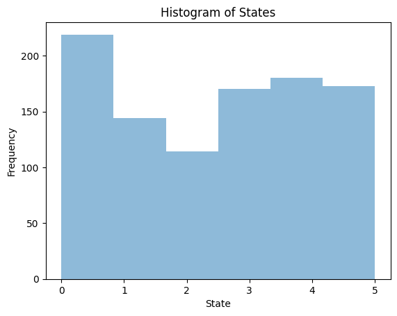
Comparing the theoretical and emperical results
# Plotting the histogram of states
plt.hist(states, bins=6, density=True, alpha=0.7, label='Empirical')

# Plotting the stationary distribution
plt.plot(stationary_distribution, label='Theoretical', marker='o')

plt.title('Comparison of Empirical and Theoretical Distributions')
plt.xlabel('States')
plt.ylabel('Probability')
plt.legend()

plt.show()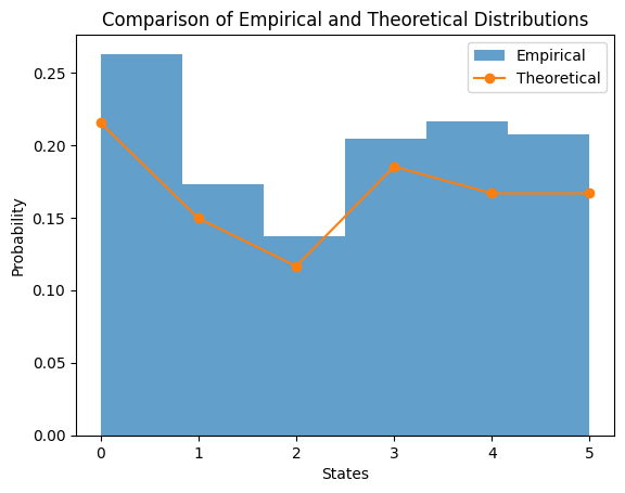
Watching the emperical distribution develop over time
import numpy as np
from IPython.display import HTML
import matplotlib.pyplot as plt
import matplotlib.animation as animation
# Use stochastic_matrix as the transition matrix
Q = stochastic_matrix
# Initialize the figure
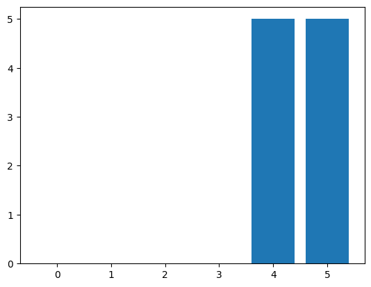
fig, ax = plt.subplots()
num_frames=100;
# Initialize an empty array for the empirical distribution
empirical_distribution = np.zeros((num_frames, len(Q[0])))
# Initialize the state variable
state = 0
# Function to update the empirical distribution
# Modify the update function to run 10 iterations without updating i
def update(i):
global state, empirical_distribution
empirical_distribution[i] = empirical_distribution[i-1]
for _ in range(10): # Run 10 iterations
state = np.random.choice(range(len(Q[state])), p=Q[state])
empirical_distribution[i, state] += 1
# Plot the distribution
ax.clear()
ax.bar(range(len(Q[state])), empirical_distribution[i] )
# Create the animation
ani = animation.FuncAnimation(fig, update, frames=range(1, num_frames), repeat=False)
# Use the HTML object to display the animation
HTML(ani.to_jshtml())