\(\displaystyle \left[\begin{matrix}56753.6889897841\\8626.56072644719\\4.02951191827469\end{matrix}\right]\)
Intro to linear systems
Linear systems
What are linear systems?
- Set of one or more linear equations involving the same variables.
- Each equation can be be put in form \(a_1 x_1 + a_2 x_2 + \dots + a_n x_n+ b = 0\)
. . .
\[ \begin{cases} a_{11} x_1 + a_{12} x_2 +\dots + a_{1n} x_n = b_1 \\ a_{21} x_1 + a_{22} x_2 + \dots + a_{2n} x_n = b_2 \\ \vdots\\ a_{m1} x_1 + a_{m2} x_2 + \dots + a_{mn} x_n = b_m, \end{cases} \]
Example: railroad cars
A chemical manufacturer wants to lease a fleet of 24 railroad tank cars with a combined carrying capacity of 520,000 gallons.
- Tank cars with three different carrying capacities are available:
- 8,000 gallons
- 16,000 gallons
- 24,000 gallons.
- How many of each type of tank car should be leased?
Example: traffic flow.

- Numbers = # of vehicles/hr that enter and leave on that street.
- \(x_{1}, x_{2}, x_{3}\), and \(x_{4}\): flow of traffic between the four intersections.
- Number of vehicles entering each intersection should always equal the number leaving. E.g.:
- 1,500 vehicles enter the intersection of 5th Street and Washington Avenue each hour
- \(x_{1}+x_{4}\) vehicles leave this intersection
- \(\rightarrow\) \(x_{1}+x_{4}=1,500\)
- Find the traffic flow at each of the other three intersections.
- What is the # of vehicles that travel from Washington Avenue to Lincoln Avenue on 5th Street?
Example: US population
- The U.S. population was approximately 75 million in 1900, 150 million in 1950, and 275 million in 2000.
- Find a quadratic equation whose graph passes through the points \((0,75)\), \((50,150)\), \((100,275)\)
. . .
Call the years \((0, 50, 100)\) \(t_i\). Call the populations \((75,150,275)\) \(y_i\).
Then we have
\[ \begin{cases} c_1 t_1 + c_2 t_1^2 = y_1 \\ c_1 t_2 + c_2 t_2^2 = y_2 \\ c_1 t_3 + c_2 t_3^2 = y_3 \end{cases} \]
. . .
Make the substitutions \(c_i \rightarrow x_i\) and \(t_i \rightarrow a_{1i}\) and \(t^2_i \rightarrow a_{2i}\), then this becomes
\[ \begin{cases} x_1 a_{11} + x_2 a_{21} =a_{11} x_1 + a_{21} x_2 = y_1 \\ x_1 a_{12} + x_2 a_{22} =a_{12} x_1 +a_{22} x_2 = y_2 \\ x_1 a_{13} + x_2 a_{23} = a_{13} x_1 + a_{23} x_2 = y_3 \end{cases} \]
We see that we now have a standard system of linear equations.
Solving linear systems
Goals for solving algorithms
An algorithm should be:
- feasible
- accurate
- stable
- efficient
- reusable computations
Example: very simple linear system
\[ \begin{gather*} 2 x-y=1 \\ 4x+4y=20 . \tag{1.5} \end{gather*} \]
. . .
Make an augmented matrix to represent the problem:
\[ \begin{aligned} & x \quad y=r . h . s . \\ & {\left[\begin{array}{rrr} 2 & -1 & 1 \\ 4 & 4 & 20 \end{array}\right]} \end{aligned} \]
. . .
Manipulate the augmented matrix to solve the problem…
Elementary Matrix Operations
When we do these on augmented matrices, the solutions are unchanged…
- \(E_{i j}\) : Swap: Switch the \(i\)th and \(j\) th rows of the matrix.
- \(E_{i}(c)\) : Scale: Multiply the \(i\)th row by the nonzero constant \(c\).
- \(E_{i j}(d)\) : Add: Add \(d\) times the \(j\)th row to the \(i\)th row.
Reduced Row Echelon Form
Every matrix can be reduced by a sequence of elementary row operations to one and only one reduced row echelon form:
- Nonzero rows of \(R\) precede the zero rows.
- Column numbers of the leading entries of the nonzero rows, say rows \(1,2, \ldots, r\), form an increasing sequence of numbers \(c_{1}<c_{2}<\cdots<c_{r}\).
- Each leading entry is a 1.
- Each leading entry has only zeros above it.
Use elementary ops to get reduced row echelon form
Gauss-Jordan elimination
- Swap rows to get non-zero number in row 1, column
- Get a 1 in the row 1, column 1.
- Make all other entries in column 1 0.
- Swap rows to get non-zero number in row 2, column 2. Make this entry 1. Make all other entries in column 2 0.
- Repeat step 4 for row 3, column 3. Continue moving along the main diagonal until you reach the last row, or until the number is zero.
. . .
Vocabulary: process of getting a 1 in a location, and then making all other entries zeros in that column, is pivoting.
The number that is made a 1 is called the pivot element, and the row that contains the pivot element is called the pivot row.
G-J Elimination for our toy system
\[ \left[\begin{array}{rrr} 4 & 4 & 20 \\ 2 & -1 & 1 \end{array}\right] \overrightarrow{E_{1}(\frac{1}{4}}\left[\begin{array}{lll} 1 & 1 & 5 \\ 2 & -1 & 1 \end{array}\right] \overrightarrow{E_{12}(-2)}\left[\begin{array}{lll} 1 & 1 & 5 \\ 0 & -3 & -9 \end{array}\right] \]
and then…
. . .
\[ \left[\begin{array}{rrr} 1 & 1 & 5 \\ 0 & -3 & -9 \end{array}\right] \overrightarrow{E_{2}(-1 / 3)}\left[\begin{array}{lll} 1 & 1 & 5 \\ 0 & 1 & 3 \end{array}\right] \overrightarrow{E_{12}(-1)}\left[\begin{array}{lll} 1 & 0 & 2 \\ 0 & 1 & 3 \end{array}\right] . \]
. . .
Writing this back as a linear system, we have:
\[ \begin{gather*} 2 x-y=1 \\ 4 x+4 y=20 \end{gather*} \Longrightarrow {\begin{aligned} & 1 \cdot x+0 \cdot y=2 \\ & 0 \cdot x+1 \cdot y=3 \end{aligned}} \Longrightarrow {\begin{aligned}x &= 2 \\ y &= 3 \end{aligned}} \]
Now you try: birds in a tree
There are 2 trees in a garden (tree “A” and “B”) and in both trees are some birds.
The birds of tree A say to the birds of tree B that if one of you comes to our tree, then our population will be double yours.
Then the birds of tree B tell the birds of tree A that if one of you comes here, then our population will be equal to yours.
How many birds in each tree?
(Solve by making an augmented matrix and doing G-J elimination.)
https://www.mathsisfun.com/puzzles/birds-in-trees.html
Example: Mining
Meyer Ch 1.5
A mine produces silica, iron, and gold
Needs Money (in $$), operating time (in hours), and labor (in person-hours).
1 pound of silica needs: $.0055, . 0011 hours of operating time, and .0093 hours of labor.
1 pound of iron needs: $.095, . 01 operating hours, and .025 labor hours.
1 pound of gold needs: $ 960, 112 operating hours, and 560 labor hours.
Suppose that during 600 hours of operation, exactly $ 5000 and 3000 labor-hours are used.
How much silica (\(x\)), iron (\(y\)), and gold (\(z\)) were produced?
. . .
Set up the linear system whose solution will yield the values for \(x, y\), and \(z\).
. . .
\[ \begin{aligned} .0055 x + .095 y + 960 z &= 5000 \quad \text{(dollars)}\\ .0011 x + .01 y + 112 z &= 600 \quad \text{(operating hours)}\\ .0093 x + .025 y + 560 z &= 3000\quad \text{(labor hours)} \end{aligned} \]
. . .
Make the augmented matrix:
\[ \left[\begin{array}{@{}ccc|c@{}} .0055 & .095 & 960 & 5000 \\ .0011 & .01 & 112 & 600 \\ .0093 & .025 & 560 & 3000 \end{array}\right] \]
We can solve this using Gauss-Jordan elimination.
Getting into row echelon form, rounding after 3 digits
\[\left[\begin{matrix}0.0055 & 0.095 & 960 & 5000\\0.0011 & 0.01 & 112 & 600\\0.0093 & 0.025 & 560 & 3000\end{matrix}\right] \overrightarrow{E_{12}(\frac{-1}{5})} \left[\begin{matrix}0.0055 & 0.095 & 9.6 \cdot 10^{2} & 5.0 \cdot 10^{3}\\0 & -0.009 & -80.0 & -4.0 \cdot 10^{2}\\0.0093 & 0.025 & 5.6 \cdot 10^{2} & 3.0 \cdot 10^{3}\end{matrix}\right]\]
\[\overrightarrow{E_{13}(\frac{93}{55})} \left[\begin{matrix}0.0055 & 0.095 & 9.6 \cdot 10^{2} & 5.0 \cdot 10^{3}\\0 & -0.009 & -80.0 & -4.0 \cdot 10^{2}\\0 & -0.14 & -1.1 \cdot 10^{3} & -5.4 \cdot 10^{3}\end{matrix}\right]\]
\[\overrightarrow{E_{23}(\frac{-14}{.9})} \left[\begin{matrix}0.0055 & 0.095 & 9.6 \cdot 10^{2} & 5.0 \cdot 10^{3}\\0 & -0.009 & -80.0 & -4.0 \cdot 10^{2}\\0 & 0 & 1.4 \cdot 10^{2} & 5.7 \cdot 10^{2}\end{matrix}\right]\]
This has solutions \(\left[\begin{matrix}5.7 \cdot 10^{4}\\8.9 \cdot 10^{3}\\4.0\end{matrix}\right]\).
. . .
How do these compare to the exact solutions? These are
Doing it again, rounding after 15 digits
\(\left[\begin{matrix}0.0055 & 0.095 & 960 & 5000\\0.0011 & 0.01 & 112 & 600\\0.0093 & 0.025 & 560 & 3000\end{matrix}\right] \rightarrow \left[\begin{matrix}0.0055 & 0.095 & 960.0 & 5000.0\\0 & -0.009 & -80.0 & -400.0\\0.0093 & 0.025 & 560.0 & 3000.0\end{matrix}\right]\)
\(\rightarrow \left[\begin{matrix}0.0055 & 0.095 & 960.0 & 5000.0\\0 & -0.009 & -80.0 & -400.0\\0 & -0.135636363636364 & -1063.27272727273 & -5454.54545454545\end{matrix}\right] \rightarrow \left[\begin{matrix}0.0055 & 0.095 & 960.0 & 5000.0\\0 & -0.009 & -80.0 & -400.0\\0 & 0 & 142.383838383838 & 573.737373737372\end{matrix}\right]\)
This has solutions \(\left[\begin{matrix}56753.6889897845\\8626.56072644727\\4.02951191827468\end{matrix}\right]\).
Reminder, the exact solution was:
\(\displaystyle \left[\begin{matrix}56753.6889897841\\8626.56072644719\\4.02951191827469\end{matrix}\right]\)
Comparing the G-J algorithm with our goals
Reminder of goals
An algorithm should be:
- feasible
- accurate
- stable
- efficient
- reusable computations
Roundoff errors
Roundoff errors with G-J elimination
Try this on your calculator. What do you get?
\[ \left(\left(\frac{2}{3}+100\right)-100\right)-\frac{2}{3}\stackrel{?}{=}0 \]
. . .
Now try this…
\[ \left(\left(\frac{2}{3}+100\right)-100\right)-\frac{2}{3}\stackrel{?}{=}0 \]
Let \(\epsilon\) be a number so small that our calculator yields \(1+\epsilon=1\).
With this calculator, \(1+1 / \epsilon=(\epsilon+1) / \epsilon=1 / \epsilon\)
Want to solve the linear system
\[ \begin{align*} \epsilon x_{1}+x_{2} & =1\\ x_{1}-x_{2} & =0 . \end{align*} \]
Roundoff errors with G-J elimination
With our calculator,
\[ \left[\begin{array}{rrr} \epsilon & 1 & 1 \\ 1 & -1 & 0 \end{array}\right] \overrightarrow{E_{21}\left(-\frac{1}{\epsilon}\right)}\left[\begin{array}{ccc} \epsilon & 1 & 1 \\ 0 & \frac{1}{\epsilon} & -\frac{1}{\epsilon} \end{array}\right] \overrightarrow{E_{2}(\epsilon)}\left[\begin{array}{ccc} \epsilon & 1 & 1 \\ 0 & 1 & 1 \end{array}\right] \\ \overrightarrow{E_{12}(-1)}\left[\begin{array}{ccc} \epsilon & 0 & 0 \\ 0 & 1 & 1 \end{array}\right] \overrightarrow{E_{1}\left(\frac{1}{\epsilon}\right)}\left[\begin{array}{lll} 1 & 0 & 0 \\ 0 & 1 & 1 \end{array}\right] . \]
. . .
Calculated solution: \(x_{1}=0, x_{2}=1\)
Correct answer should be
\[ x_{1}=x_{2}=\frac{1}{1+\epsilon}=0.999999099999990 \ldots\]
Sensitivity to small changes
Problem arose because we took a computational step where we added two numbers of very different scale, essentially losing the smaller number.
Led to a big changes in output!
There is no general cure for these difficulties…
Want to be aware of them, know when we are doing computations that might be susceptible.
Partial pivoting
We can improve performance of G-J by introducing a new step into the algorithm:
Find the entry in the left column with the largest absolute value. This entry is called the pivot. Perform row interchange (if necessary), so that the pivot is in the first row.
Use a row operation to get a 1 as the entry in the first row and first column.
Use row operations to make all other entries as zeros in column one.
Interchange rows if necessary to obtain a nonzero number with the largest absolute value in the second row, second column. Use a row operation to make this entry 1. Use row operations to make all other entries as zeros in column two.
Repeat step 4 for row 3, column 3. Continue moving along the main diagonal until you reach the last row, or until the number is zero.
Using partial pivoting in our example
Ill-conditioned linear systems
Ill-conditioned linear systems
A system of linear equations is said to be ill-conditioned when some small perturbation in the system (in the \(b\)s) can produce relatively large changes in the exact solution (in the \(x\)’s). Otherwise, the system is said to be well-conditioned.
Ill-conditioned linear systems
Meyer Ch 1.6
Consider \[ \begin{aligned} & .835 x+.667 y=.168, \\ & .333 x+.266 y=.067, \end{aligned} \]
Exact solution:
\[ x=1 \quad \text { and } \quad y=-1 . \]
But if we change just one digit…
\[ \begin{aligned} & .835 x+.667 y=.168, \\ & .333 x+.266 y=.06\color{red}{6}, \end{aligned} \]
Now exact solution:
\[ \hat{x}=-666 \quad \text { and } \quad \hat{y}=834 \]
What if \(b_1\) and \(b_2\) are the results of an experiment, need to be read off a dial? Suppose:
- dial can be read to tolerance of \(\pm .001\),
- values for \(b_{1}\) and \(b_{2}\) are read as .168 and .067, respectively. Then the exact solution is
\[ \begin{equation*} (x, y)=(1,-1) \end{equation*} \]
- But due to uncertainty, we have
\[ \begin{equation*} .167 \leq b_{1} \leq .169 \quad \text { and } \quad .066 \leq b_{2} \leq .068 \end{equation*} \]
| \(b_1\) | \(b_2\) | \(x\) | \(y\) |
|---|---|---|---|
| .168 | .067 | 1 | -1 |
| .167 | .068 | 934 | -1169 |
| .169 | .066 | -932 | 1169 |
Geometrical interpretation
If two straight lines are almost parallel and if one of the lines is moved only slightly, then the point of intersection is drastically altered.

The point of intersection is the solution of the associated \(2 \times 2\) linear system, so this is also drastically altered.
- Often in real life, coefficients are empirically obtained
- Will be off from “true” values by small amounts
- For ill-conditioned systems, this means that solutions can be very far off from true solutions
- We’ll cover techniques for quantifying conditioning, later in quarter
- For now, can just try making small changes to some coefficients. Big changes in result? Ill-conditioned system!
Example: Polynomial interpolation
Polynomial interpolation
https://colab.research.google.com/github/quantecon/lecture-julia.notebooks/blob/main/tools_and_techniques/iterative_methods_sparsity.ipynb#scrollTo=9aa1791b
Suppose we’d like to find a polynomial that can interpolate a given function.
Take points 𝑥0,…𝑥𝑁 and values 𝑦0,…𝑦𝑁
Simple way: finding the coefficients $ c_1, c_n $ where
\[ P(x) = \sum_{i=0}^N c_i x^i \]
. . .
This is a system of equations:
\[ \begin{array} cy_0 = c_0 + c_1 x_0 + \ldots c_N x_0^N\\ \,\ldots\\ \,y_N = c_0 + c_1 x_N + \ldots c_N x_N^N \end{array} \]
Polynomial interpolation
Or, stacking, \(c = \begin{bmatrix} c_0 & \ldots & c_N\end{bmatrix}\), \(y = \begin{bmatrix} y_0 & \ldots & y_N\end{bmatrix}\) , and
\[ A = \begin{bmatrix} 1 & x_0 & x_0^2 & \ldots &x_0^N\\ \vdots & \vdots & \vdots & \vdots & \vdots \\ 1 & x_N & x_N^2 & \ldots & x_N^N \end{bmatrix} \]
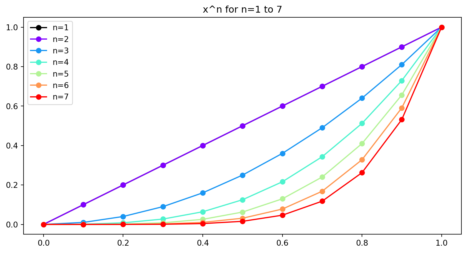
Let’s try solving this for a simple function, \(y=exp(x)\).
Polynomial interpolation
\[ x*y \]
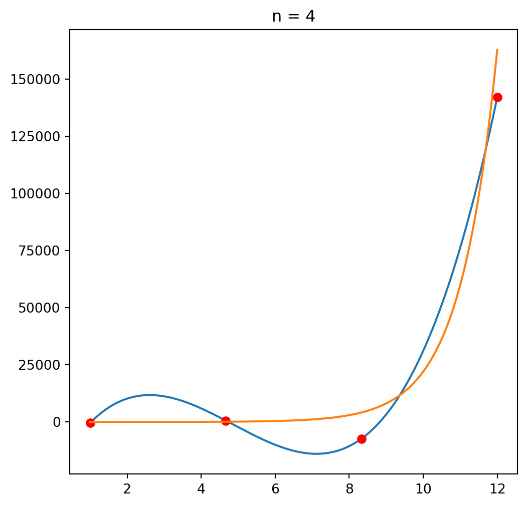
We’ll start with picking 4 interpolating points: \(\vec x = \mathtt{\text{[ 1. 4.66666667 8.33333333 12. ]}}\). Then we have our matrix A:
\[A = \begin{bmatrix} 1 & x_0 & x_0^2 & \ldots &x_0^N\\ \vdots & \vdots & \vdots & \vdots & \vdots \\ 1 & x_N & x_N^2 & \ldots & x_N^N \end{bmatrix} = \left[\begin{matrix}1.0 & 1.0 & 1.0 & 1.0\\1.0 & 4.66666666666667 & 21.7777777777778 & 101.62962962963\\1.0 & 8.33333333333333 & 69.4444444444444 & 578.703703703703\\1.0 & 12.0 & 144.0 & 1728.0\end{matrix}\right] \]
Our \(y\) values are \(\vec y = \mathtt{\text{[ 2.71828183 106.3426754 4160.26200538 162754.791419 ]}}\). We could solve this using Gauss-Jordan elimination, or here the solving algorithm built into Numpy.
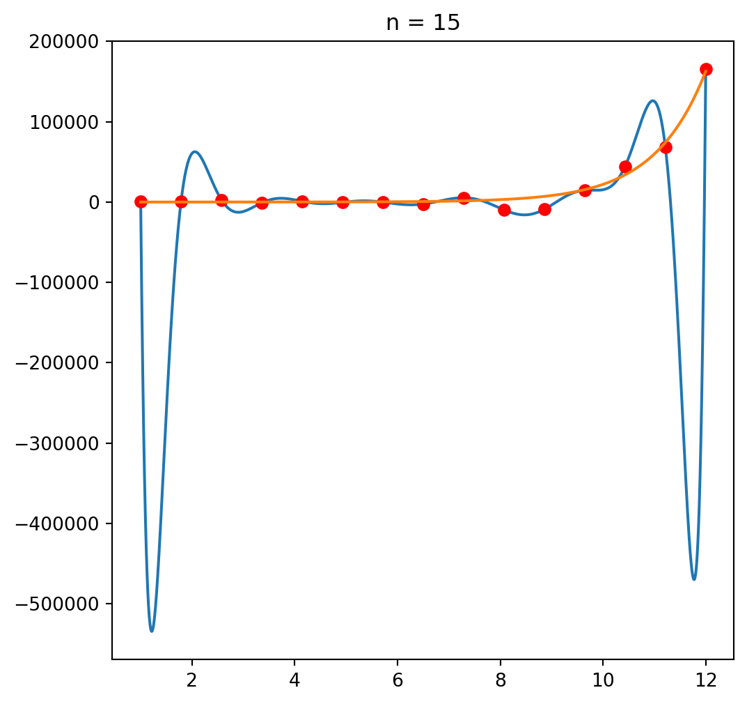
Results for n=4 and n=10 points
Max error for different values of n
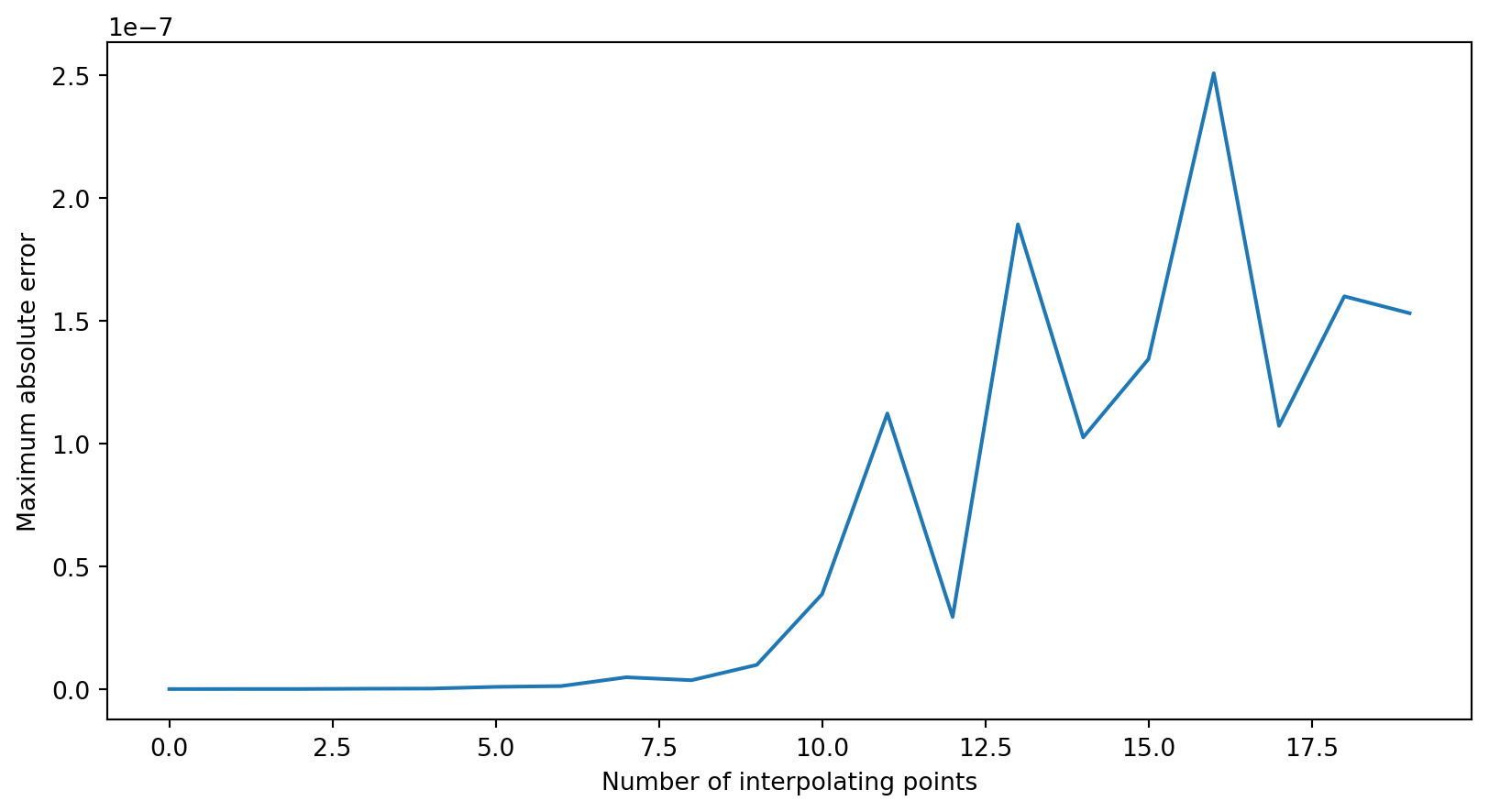
The problem: linear dependency