Ch2 Lecture 1

Reaction-Diffusion Equations

Diffusion

Adapted from this blog post.

Last week, we talked about the diffusion equation. Here is the exact form:

\[\frac{\partial a(x,t)}{\partial t} = D_{a}\frac{\partial^{2} a(x,t)}{\partial x^{2}}\]

. . .

We approximated this using the finite-difference method:

Time derivative (which we had set to zero):

\[ \frac{\partial a(x,t)}{\partial t} \approx \frac{1}{dt}(a_{x,t+1} - a_{x,t}) \]

Spacial part of the derivative (which is usually know as the Laplacian):

\[ \frac{\partial^{2} a(x,t)}{\partial x^{2}} \approx \frac{1}{dx^{2}}(a_{x+1,t} + a_{x-1,t} - 2a_{x,t}) \]

. . .

This gives us the finite-difference equation:

\[ a_{x,t+1} = a_{x,t} + dt\left( \frac{D_{a}}{dx^{2}}(a_{x+1,t} + a_{x-1,t} - 2a_{x,t}) \right) \]

Boundary Conditions

• Last week, with our metal rod, we had boundary conditions where the temperatures at the ends of the rod were fixed at 0 degrees.

• We needed to say something about the boundaries to solve the system of equations.

• Another option is periodic boundary conditions.

• These are like imagining the rod is a loop, so the temperature at the end of the rod is the same as the temperature at the beginning of the rod.

Periodic Boundary Conditions: np.roll

• Want an easy way to compute \(a_{x+1}\) for all \(x\)’s

• Suppose we have n points, and we want to compute \(a_{x+1}\) for all \(x\)=n.

• Problem: \(a_{x+1}\) would be off the end of the array!

• Just replace \(a_{n+1}\) with \(a_{1}\)

• Can do this easily with np.roll. Lets us compute \(a_{x+1}\) for all \(x\)’s.

. . .

Laplacian with Periodic Boundary Conditions in Python

import numpy as np
def laplacian1D(a, dx):
    return (
        - 2 * a
        + np.roll(a,1,axis=0)
        + np.roll(a,-1,axis=0)
    ) / (dx ** 2)

def laplacian2D(a, dx):
    return (
        - 4 * a
        + np.roll(a,1,axis=0)
        + np.roll(a,-1,axis=0)
        + np.roll(a,+1,axis=1)
        + np.roll(a,-1,axis=1)
    ) / (dx ** 2)

The autoreload extension is already loaded. To reload it, use:
  %reload_ext autoreload

Solving and animating

class OneDimensionalDiffusionEquation(BaseStateSystem):
    def __init__(self, D):
        self.D = D
        self.width = 1000
        self.dx = 10 / self.width
        self.dt = 0.9 * (self.dx ** 2) / (2 * D)
        self.steps = int(0.1 / self.dt)

    def initialise(self):
        self.t = 0
        self.X = np.linspace(-5,5,self.width)
        self.a = np.exp(-self.X**2)

    def update(self):
        for _ in range(self.steps):
            self.t += self.dt
            self._update()

    def _update(self):
        La = laplacian1D(self.a, self.dx)
        delta_a = self.dt * (self.D * La)
        self.a += delta_a

    def draw(self, ax):
        ax.clear()
        ax.plot(self.X,self.a, color="r")
        ax.set_ylim(0,1)
        ax.set_xlim(-5,5)
        ax.set_title("t = {:.2f}".format(self.t))

one_d_diffusion = OneDimensionalDiffusionEquation(D=1)

one_d_diffusion.plot_time_evolution("diffusion.gif")

diffusion.gif

Reaction Terms

• We will have a system with two chemical components, \(a\) and \(b\).

• Suppose \(a\) activates genes which produce pigmentation. \(b\) inhibits \(a\)

• Will start with some random small initial concentrations of \(a\) and \(b\).

• Each will diffuse according to the diffusion equation.

• They will also react with each other, changing the concentration of each.

. . .

For the reaction equations, will use the FitzHugh–Nagumo equation

\(R_a(a, b) = a - a^{3} - b + \alpha\)

\(R_{b}(a, b) = \beta (a - b)\)

Where \(\alpha\) and \(\beta\) are constants.

Reaction Equation evolution at one point in space

class ReactionEquation(BaseStateSystem):
    def __init__(self, Ra, Rb):
        self.Ra = Ra
        self.Rb = Rb
        self.dt = 0.01
        self.steps = int(0.1 / self.dt)

    def initialise(self):
        self.t = 0
        self.a = 0.1
        self.b = 0.7
        self.Ya = []
        self.Yb = []
        self.X = []

    def update(self):
        for _ in range(self.steps):
            self.t += self.dt
            self._update()

    def _update(self):
        delta_a = self.dt * self.Ra(self.a,self.b)
        delta_b = self.dt * self.Rb(self.a,self.b)

        self.a += delta_a
        self.b += delta_b

    def draw(self, ax):
        ax.clear()

        self.X.append(self.t)
        self.Ya.append(self.a)
        self.Yb.append(self.b)

        ax.plot(self.X,self.Ya, color="r", label="A")
        ax.plot(self.X,self.Yb, color="b", label="B")
        ax.legend()

        ax.set_ylim(0,1)
        ax.set_xlim(0,5)
        ax.set_xlabel("t")
        ax.set_ylabel("Concentrations")

alpha, beta =  0.2, 5

def Ra(a,b): return a - a ** 3 - b + alpha
def Rb(a,b): return (a - b) * beta

one_d_reaction = ReactionEquation(Ra, Rb)
one_d_reaction.plot_time_evolution("reaction.gif", n_steps=50)

reaction.gif

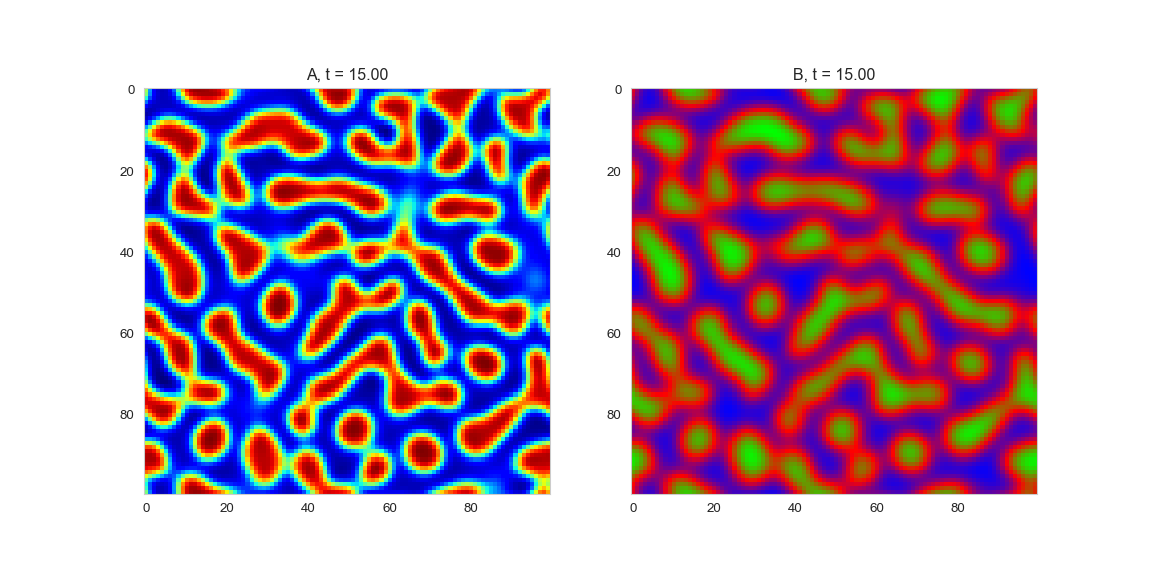
Full Model

We now have two parts: - a diffusion term that “spreads” out concentration - a reaction part the equalises the two concentrations. . . .

What happens when we put the two together? Do we get something stable?

def random_initialiser(shape):
    return(
        np.random.normal(loc=0, scale=0.05, size=shape),
        np.random.normal(loc=0, scale=0.05, size=shape)
    )

class OneDimensionalRDEquations(BaseStateSystem):
    def __init__(self, Da, Db, Ra, Rb,
                 initialiser=random_initialiser,
                 width=1000, dx=1,
                 dt=0.1, steps=1):

        self.Da = Da
        self.Db = Db
        self.Ra = Ra
        self.Rb = Rb

        self.initialiser = initialiser
        self.width = width
        self.dx = dx
        self.dt = dt
        self.steps = steps

    def initialise(self):
        self.t = 0
        self.a, self.b = self.initialiser(self.width)

    def update(self):
        for _ in range(self.steps):
            self.t += self.dt
            self._update()

    def _update(self):

        # unpack so we don't have to keep writing "self"
        a,b,Da,Db,Ra,Rb,dt,dx = (
            self.a, self.b,
            self.Da, self.Db,
            self.Ra, self.Rb,
            self.dt, self.dx
        )

        La = laplacian1D(a, dx)
        Lb = laplacian1D(b, dx)

        delta_a = dt * (Da * La + Ra(a,b))
        delta_b = dt * (Db * Lb + Rb(a,b))

        self.a += delta_a
        self.b += delta_b

    def draw(self, ax):
        ax.clear()
        ax.plot(self.a, color="r", label="A")
        ax.plot(self.b, color="b", label="B")
        ax.legend()
        ax.set_ylim(-1,1)
        ax.set_title("t = {:.2f}".format(self.t))

Da, Db, alpha, beta = 1, 100, -0.005, 10

def Ra(a,b): return a - a ** 3 - b + alpha
def Rb(a,b): return (a - b) * beta

width = 100
dx = 1
dt = 0.001

OneDimensionalRDEquations(
    Da, Db, Ra, Rb,
    width=width, dx=dx, dt=dt,
    steps=100
).plot_time_evolution("1dRD.gif", n_steps=150)

1dRD.gif

In two dimensions

2dRD.png

Review of Matrix Arithmetic

Matrix Addition and Subtraction

Review matrix addition and subtraction on your own!

Matrix Multiplication

For motivation:

\[ 2 x-3 y+4 z=5 \text {. } \]

• Can write as a “product” of the coefficient matrix \([2,-3,4]\) and and the column matrix of unknowns \(\left[\begin{array}{l}x \\ y \\ z\end{array}\right]\).

. . .

Thus, product is:

\[ [2,-3,4]\left[\begin{array}{l} x \\ y \\ z \end{array}\right]=[2 x-3 y+4 z] \]

Definition of matrix product

\(A=\left[a_{i j}\right]\): \(m \times p\) matrix

\(B=\left[b_{i j}\right]\): \(p \times n\) matrix.

Product of \(A\) and \(B\) – \(A B\)

• is \(m \times n\) matrix whose
• \((i, j)\) th entry is the entry of the product of the \(i\) th row of \(A\) and the \(j\) th column of \(B\);

. . .

More specifically, the \((i, j)\) th entry of \(A B\) is

\[ a_{i 1} b_{1 j}+a_{i 2} b_{2 j}+\cdots+a_{i p} b_{p j} . \]

Reminder: Matrix Multiplication is not Commutative

• \(A B \neq B A\) in general.

Linear Systems as a Matrix Product

We can express a linear system of equations as a matrix product:

\[ \begin{aligned} x_{1}+x_{2}+x_{3} & =4 \\ 2 x_{1}+2 x_{2}+5 x_{3} & =11 \\ 4 x_{1}+6 x_{2}+8 x_{3} & =24 \end{aligned} \]

. . .

\[ \mathbf{x}=\left[\begin{array}{l} x_{1} \\ x_{2} \\ x_{3} \end{array}\right], \quad \mathbf{b}=\left[\begin{array}{r} 4 \\ 11 \\ 24 \end{array}\right], \quad \text { and } A=\left[\begin{array}{lll} 1 & 1 & 1 \\ 2 & 2 & 5 \\ 4 & 6 & 8 \end{array}\right] \]

. . .

\[ A \mathbf{x}=\left[\begin{array}{lll} 1 & 1 & 1 \\ 2 & 2 & 5 \\ 4 & 6 & 8 \end{array}\right]\left[\begin{array}{l} x_{1} \\ x_{2} \\ x_{3} \end{array}\right]=\left[\begin{array}{r} 4 \\ 11 \\ 24 \end{array}\right]=\mathbf{b} \]

Matrix Multiplication as a Linear Combination of Column Vectors

Another way of writing this system:

\[ x_{1}\left[\begin{array}{l} 1 \\ 2 \\ 4 \end{array}\right]+x_{2}\left[\begin{array}{l} 1 \\ 2 \\ 6 \end{array}\right]+x_{3}\left[\begin{array}{l} 1 \\ 5 \\ 8 \end{array}\right]=\left[\begin{array}{r} 4 \\ 11 \\ 24 \end{array}\right] . \]

. . .

Name the columns of A as \(\mathbf{a_1}, \mathbf{a_2}, \mathbf{a_3}\), then we can write the matrix as \(A=\left[\mathbf{a}_{1}, \mathbf{a}_{2}, \mathbf{a}_{3}\right]\)

. . .

Let \(\mathbf{x}=\left(x_{1}, x_{2}, x_{3}\right)\). Then

\[ A \mathbf{x}=x_{1} \mathbf{a}_{1}+x_{2} \mathbf{a}_{2}+x_{3} \mathbf{a}_{3} . \]

This is a very important way of thinking about matrix multiplication

Try it yourself

Try to find the solution for the following system, by trying different values of \(x_i\) to use in a sum of the columns of \(A\).

\[ A \mathbf{x} = \left[\begin{array}{lll} 1 & 1 & 1 \\ 2 & 2 & 5 \\ 4 & 6 & 8 \end{array}\right]\left[\begin{array}{l} x_1 \\ x_2 \\ x_3 \end{array}\right]=x_{1} \mathbf{a}_{1}+x_{2} \mathbf{a}_{2}+x_{3} \mathbf{a}_{3} =\left[\begin{array}{l} 6 \\ 21 \\ 38 \end{array}\right] \]

. . .

Now try changing the right-hand side to a different vector. Can you still find a solution? (You may need to use non-integer values for the \(x\)’s.)

This is a slightly changed system.

\[ A \mathbf{x} = \left[\begin{array}{lll} 1 & 1 & 2 \\ 1 & 2 & 2 \\ 4 & 6 & 8 \end{array}\right]\left[\begin{array}{l} x_1 \\ x_2 \\ x_3 \end{array}\right]=x_{1} \mathbf{a}_{1}+x_{2} \mathbf{a}_{2}+x_{3} \mathbf{a}_{3} =\left[\begin{array}{l} 11 \\ 12 \\ 46 \end{array}\right] \]

. . .

Are you able to find more than one solution? Can you find a right-hand-side that doesn’t have a solution?

Example: Benzoic acid

Benzoic acid (chemical formula \(\mathrm{C}_{7} \mathrm{H}_{6} \mathrm{O}_{2}\) ) oxidizes to carbon dioxide and water.

\[ \mathrm{C}_{7} \mathrm{H}_{6} \mathrm{O}_{2}+\mathrm{O}_{2} \rightarrow \mathrm{CO}_{2}+\mathrm{H}_{2} \mathrm{O} . \]

Balance this equation. (Make the number of atoms of each element match on the two sides of the equation.)

. . .

Define \((c, o, h)\) as the number of atoms of carbon, oxygen, and hydrogen atoms in the equation.

. . .

Next let \(x_1\), \(x_2\), \(x_3\), and \(x_4\) be the number of molecules of benzoic acid, oxygen, carbon dioxide, and water, respectively.

. . .

Then we have the equation

\[ x_{1}\left[\begin{array}{l} 7 \\ 2 \\ 6 \end{array}\right]+x_{2}\left[\begin{array}{l} 0 \\ 2 \\ 0 \end{array}\right]=x_{3}\left[\begin{array}{l} 1 \\ 2 \\ 0 \end{array}\right]+x_{4}\left[\begin{array}{l} 0 \\ 1 \\ 2 \end{array}\right] . \]

Rearrange:

\[ x_{1}\left[\begin{array}{l} 7 \\ 2 \\ 6 \end{array}\right]+x_{2}\left[\begin{array}{l} 0 \\ 2 \\ 0 \end{array}\right]=x_{3}\left[\begin{array}{l} 1 \\ 2 \\ 0 \end{array}\right]+x_{4}\left[\begin{array}{l} 0 \\ 1 \\ 2 \end{array}\right] . \]

becomes

\[ A \mathbf{x}=\left[\begin{array}{cccc} 7 & 0 & -1 & 0 \\ 2 & 2 & -2 & -1 \\ 6 & 0 & 0 & -2 \end{array}\right]\left[\begin{array}{l} x_{1} \\ x_{2} \\ x_{3} \\ x_{4} \end{array}\right]=\left[\begin{array}{l} 0 \\ 0 \\ 0 \end{array}\right] \]

We solve with row reduction:

\[ \begin{aligned} & {\left[\begin{array}{cccc} 7 & 0 & -1 & 0 \\ 2 & 2 & -2 & -1 \\ 6 & 0 & 0 & -2 \end{array}\right] \xrightarrow[E_{21}\left(-\frac{2}{7}\right)]{E_{31}\left(-\frac{6}{7}\right)}\left[\begin{array}{cccc} 7 & 0 & -1 & 0 \\ 0 & 2 & -\frac{12}{7} & -1 \\ 0 & 0 & \frac{6}{7} & -2 \end{array}\right] \begin{array}{c} E_{1}\left(\frac{1}{7}\right) \\ E_{2}\left(\frac{1}{2}\right) \\ E_{3}\left(\frac{7}{6}\right) \end{array} \left[\begin{array}{cccc} 1 & 0 & -\frac{1}{7} & 0 \\ 0 & 1 & -\frac{6}{7} & -\frac{1}{2} \\ 0 & 0 & 1 & -\frac{7}{3} \end{array}\right]} \\ & \begin{array}{l} \overrightarrow{E_{23}\left(\frac{6}{7}\right)} \\ E_{13}\left(\frac{1}{7}\right) \end{array}\left[\begin{array}{llll} 1 & 0 & 0 & -\frac{1}{3} \\ 0 & 1 & 0 & -\frac{5}{2} \\ 0 & 0 & 1 & -\frac{7}{3} \end{array}\right] \end{aligned} \]

. . .

\(x_{4}\) is free, others are bound. Now pick smallest \(x_4\) where others are all positive integers…

. . .

\[ 2 \mathrm{C}_{7} \mathrm{H}_{6} \mathrm{O}_{2}+15 \mathrm{O}_{2} \rightarrow 14 \mathrm{CO}_{2}+6 \mathrm{H}_{2} \mathrm{O} \]

Matrix Multiplication as a Function

Every matrix \(A\) is associated with a function \(T_A\) that takes a vector as input and returns a vector as output.

\[ T_{A}(\mathbf{u})=A \mathbf{u} \]

. . .

Other names for \(T_A\) are “linear transformation” or “linear operator”.

Transformations

Scaling

Goal: Make a matrix that will take a vector of coordinates \(\mathbf{x}\) and scale each coordinate \(x_i\) by a factor of \(z_i\).

\[ A x = \left[\begin{array}{ll} a1 & a2 \\ a3 & a4 \end{array}\right] \left[\begin{array}{l} x_1 \\ x_2 \end{array}\right] = \left[\begin{array}{l} z_1 \times x_1 \\ z_2\times x_2 \end{array}\right] \]

. . .

\[ A = \left[\begin{array}{ll} z_1 & 0 \\ 0 & z_2 \end{array}\right] \]

Shearing

Shearing: adding a constant shear factor times one coordinate to another coordinate of the point.

Goal: make a matrix which will transform each coordinate \(x_i\) into \(x_i + \sum_{j \ne i} s_{j} \times x_j\).

\[ A x = \left[\begin{array}{ll} a1 & a2 \\ a3 & a4 \end{array}\right] \left[\begin{array}{l} x_1 \\ x_2 \end{array}\right] = \left[\begin{array}{l} x_1 + s_2 x_2 \\ x_2 + s_1 x_1 \end{array}\right] \]

. . .

\[ A = \left[\begin{array}{ll} 1 & s_2 \\ s_1 & 1 \end{array}\right] \]

Example

• Let the scaling operator \(S\) on points in two dimensions have scale factors of \(\frac{3}{2}\) in the \(x\)-direction and \(\frac{1}{2}\) in the \(y\)-direction.

• Let the shearing operator \(H\) on these points have a shear factor of \(\frac{1}{2}\) by the \(y\)-coordinate on the \(x\)-coordinate.

• Express these operators as matrix operators and graph their action on four unit squares situated diagonally from the origin.

Solution

• Scaling operator \(S\):

. . .

\[ S((x, y))=\left[\begin{array}{c} \frac{3}{2} x \\ \frac{1}{2} y \end{array}\right]=\left[\begin{array}{cc} \frac{3}{2} & 0 \\ 0 & \frac{1}{2} \end{array}\right]\left[\begin{array}{l} x \\ y \end{array}\right]=T_{A}((x, y)) \]

. . .

Verify:

• Shearing operator \(H\):

\[ H((x, y))=\left[\begin{array}{c} x+\frac{1}{2} y \\ y \end{array}\right]=\left[\begin{array}{ll} 1 & \frac{1}{2} \\ 0 & 1 \end{array}\right]\left[\begin{array}{l} x \\ y \end{array}\right]=T_{B}((x, y)) \]

Verify

Concatenation of operators \(S\) and \(H\)

• The concatenation \(S \circ H\) of the scaling operator \(S\) and shearing operator \(H\) is the action of scaling followed by shearing.

• Function composition corresponds to matrix multiplication

. . .

\[ \begin{aligned} S \circ H((x, y)) & =T_{A} \circ T_{B}((x, y))=T_{A B}((x, y)) \\ & =\left[\begin{array}{cc} \frac{3}{2} & 0 \\ 0 & \frac{1}{2} \end{array}\right]\left[\begin{array}{ll} 1 & \frac{1}{2} \\ 0 & 1 \end{array}\right]\left[\begin{array}{l} x \\ y \end{array}\right]=\left[\begin{array}{cc} \frac{3}{2} & \frac{3}{4} \\ 0 & \frac{1}{2} \end{array}\right]\left[\begin{array}{l} x \\ y \end{array}\right]=T_{C}((x, y)), \end{aligned} \]

Verify

Rotation

Goal: rotate a point in two dimensions counterclockwise by an angle \(\phi\). Suppose the point is initally at an angle \(\theta\) from the \(x\)-axis.

\[ \left[\begin{array}{l} x \\ y \end{array}\right] =\left[\begin{array}{l} r \cos \theta \\ r \sin \theta \end{array}\right] \]

We can use trigonometry to find the values of x and y after rotation.

\[ \left[\begin{array}{l} x^{\prime} \\ y^{\prime} \end{array}\right] =\left[\begin{array}{l} r \cos (\theta+\phi) \\ r \sin (\theta+\phi) \end{array}\right]=\left[\begin{array}{l} r \cos \theta \cos \phi-r \sin \theta \sin \phi \\ r \sin \theta \cos \phi+r \cos \theta \sin \phi \end{array}\right] \]

. . .

Using the double-angle rule,

\[ =\left[\begin{array}{rr} \cos \theta &-\sin \theta \\ \sin \theta & \cos \theta \end{array}\right]\left[\begin{array}{l} r \cos \phi \\ r \sin \phi \end{array}\right]=\left[\begin{array}{rr} \cos \theta&-\sin \theta \\ \sin \theta & \cos \theta \end{array}\right]\left[\begin{array}{l} x \\ y \end{array}\right] \]

. . .

So we define the rotation matrix \(R(\theta)\) by

\[ R(\theta)=\left[\begin{array}{rr} \cos \theta & -\sin \theta \\ \sin \theta & \cos \theta \end{array}\right] \]

Now you try

diffusion.gif reaction.gif 1dRD.gif 2dRD.png