Ch2 Lecture 2

Discrete Dynamical Systems

Definitions

Definition: A discrete linear dynamical system is a sequence of vectors \(\mathbf{x}^{(k)}, k=0,1, \ldots\), called states, which is defined by an initial vector \(\mathbf{x}^{(0)}\) and by the rule

\[ \mathbf{x}^{(k+1)}=A \mathbf{x}^{(k)}+\mathbf{b}_{k}, \quad k=0,1, \ldots \]

. . .

\(A\) is a fixed square matrix, called the transition matrix of the system
vectors \(\mathbf{b}_{k}, k=0,1, \ldots\) are called the input vectors of the system.
If we don’t specify input vectors, assume that \(\mathbf{b}_{k}=\mathbf{0}\) for all \(k\). Then call the system a homogeneous dynamical system.

Stability

An important question: is the system stable?

Does \(\mathbf{x}^{(k)}\) tend towards a constant state \(\mathrm{x}\)?

. . .

If system is homogeneous, then if a stable state is the initial state, it will equal all subsequent states.

Definition: A vector \(\mathbf{x}\) satisfying \(\mathbf{x}=A \mathbf{x}\), for a square matrix \(A\), is called a stationary vector for \(A\).

. . .

If \(A\) is the transition matrix for a homogeneous discrete dynamical system, we also call such a vector a stationary state.

Example

Two toothpaste companies compete for customers in a fixed market
Each customer uses either Brand A or Brand B.
Buying habits. In each quarter:
- \(30 \%\) of A users will switch to B, while the rest stay with A.
- \(40 \%\) of B users will switch to A , while the the rest stay with B.
This is an example of a Markov chain model.

Let \(a_1\) be the fraction of customers using Brand A at the end of the first quarter, and \(b_1\) be the fraction using Brand B.

Then we have the following system of equations: \[ \begin{aligned} a_{1} & =0.7 a_{0}+0.4 b_{0} \\ b_{1} & =0.3 a_{0}+0.6 b_{0} \end{aligned} \]

. . .

More generally,

\[ \begin{aligned} a_{k+1} & =0.7 a_{k}+0.4 b_{k} \\ b_{k+1} & =0.3 a_{k}+0.6 b_{k} . \end{aligned} \]

. . .

In matrix form,

\[ \mathbf{x}^{(k)}=\left[\begin{array}{c} a_{k} \\ b_{k} \end{array}\right] \text { and } A=\left[\begin{array}{ll} 0.7 & 0.4 \\ 0.3 & 0.6 \end{array}\right] \]

with

\[ \mathbf{x}^{(k+1)}=A \mathbf{x}^{(k)} \]

We can continue into future quarters by multiplying by \(A\) again: \[ \mathbf{x}^{(2)}=A \mathbf{x}^{(1)}=A \cdot\left(A \mathbf{x}^{(0)}\right)=A^{2} \mathbf{x}^{(0)} \]

. . .

In general,

\[ \mathbf{x}^{(k)}=A \mathbf{x}^{(k-1)}=A^{2} \mathbf{x}^{(k-2)}=\cdots=A^{k} \mathbf{x}^{(0)} . \]

. . .

This is true of any homogeneous linear dynamical system!

For any positive integer \(k\) and discrete dynamical system with transition matrix \(A\) and initial state \(\mathbf{x}^{(0)}\), the \(k\)-th state is given by

\[ \mathbf{x}^{(k)}=A^{k} \mathbf{x}^{(0)} \]

Distribution vector and stochastic matrix

\(\mathbf{x}^{(k)}\) of the toothpaste example are column vectors with nonnegative coordinates that sum to 1.
Such vectors are called distribution vectors.
Also, each of the columns the matrix \(A\) is a distribution vector.
A square matrix \(A\) whose columns are distribution vectors is called a stochastic matrix.

Markov Chain definition

A Markov chain is a discrete dynamical system whose initial state \(\mathbf{x}^{(0)}\) is a distribution vector and whose transition matrix \(A\) is stochastic, i.e., each column of \(A\) is a distribution vector.

Checking that our toothpase example is a Markov chain

\[ \mathbf{x}^{(k)}=\left[\begin{array}{c} a_{k} \\ b_{k} \end{array}\right] \text { and } A=\left[\begin{array}{ll} 0.7 & 0.4 \\ 0.3 & 0.6 \end{array}\right] \]

Stochastic Matrix Inequality

We can define the 1-norm of a vector \(\mathbf{x}\) as \(\|\mathbf{x}\|_{1}=\sum_{i=1}^{n}\left|x_{i}\right|\).
- If all the elements of a vector are nonnegative, then \(\|\mathbf{x}\|_{1}\) is the sum of the elements.
Can show: For any stochastic matrix \(P\) and compatible vector \(\mathbf{x},\|P \mathbf{x}\|_{1} \leq\|\mathbf{x}\|_{1}\), with equality if the coordinates of \(\mathbf{x}\) are all nonnegative.
→ if a state in a Markov chain is a distribution vector (nonnegative entries and sums to 1), then the sum of the coordinates of the next state will also sum to one
→ all subsequent states in a Markov chain are themselves Markov Chain State distribution vectors.

Moving into the future

Suppose that initially Brand A has all the customers (i.e., Brand B is just entering the market). What are the market shares 2 quarters later? 20 quarters?

. . .

Initial state vector is \(\mathbf{x}^{(0)}=(1,0)\).
Now do the arithmetic to find \(\mathbf{x}^{(2)}\) : . . . \[ \begin{aligned} {\left[\begin{array}{l} a_{2} \\ b_{2} \end{array}\right] } & =\mathbf{x}^{(2)}=A^{2} \mathbf{x}^{(0)}=\left[\begin{array}{ll} 0.7 & 0.4 \\ 0.3 & 0.6 \end{array}\right]\left(\left[\begin{array}{ll} 0.7 & 0.4 \\ 0.3 & 0.6 \end{array}\right]\left[\begin{array}{l} 1 \\ 0 \end{array}\right]\right) \\ & =\left[\begin{array}{ll} 0.7 & 0.4 \\ 0.3 & 0.6 \end{array}\right]\left[\begin{array}{l} 0.7 \\ 0.3 \end{array}\right]=\left[\begin{array}{l} .61 \\ .39 \end{array}\right] . \end{aligned} \]

Toothpaste after many quarters

Now:

find the state after 2 quarters.
find the state after 20 quarters. Use matrix exponentiation: A**n
Get specific numbers if toothpaste A has 100% of the market at the beginning. (Use sym.subs())
Now what if toothpaste B has 100% at the beginning?

Example: Structured Population Model

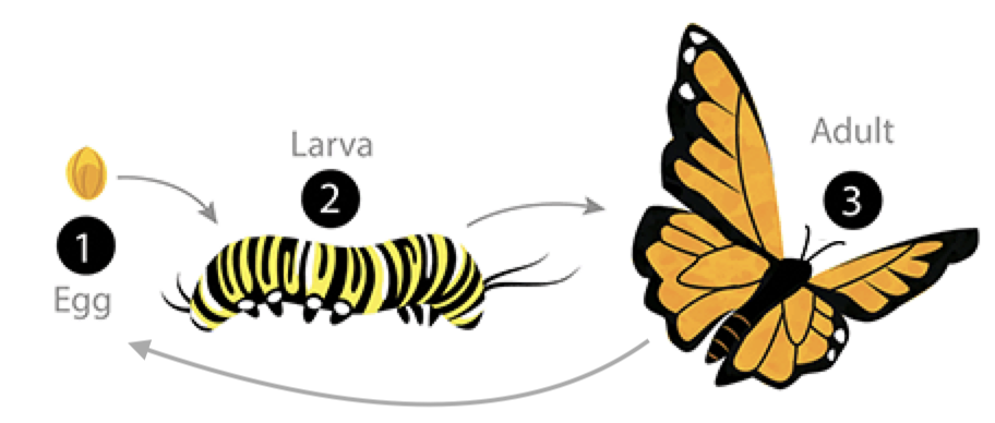
Every week, 20% of the eggs die, and 60% move to the larva stage.
Also, 10% of larvae die, 60% become adults
20% of adults die. Each adult produces 0.25 eggs.
Initially we have 10k adults, 8k larvae, 6k eggs. How does the population evolve over time?

. . .

class InsectEvolution(BaseStateSystem):
    def __init__(self,transition_matrix=np.array([[.2,0,.25],[.6,.3,0],[0,.6,.8]]),max_y=10):
        self.steps = 10;
        self.t=0
        self.transition_matrix = transition_matrix
        self.max_y=max_y

    def initialise(self):
        self.x = np.array([6,8,10])
        self.Ya = []
        self.Yb = []
        self.Yc = []
        self.X = []

    def update(self):
        for _ in range(self.steps):
            self.t += 1
            self._update()

    def _update(self):
        self.x = self.transition_matrix.dot(self.x)

    def draw(self, ax):
        ax.clear()
        self.X.append(self.t)
        self.Ya.append(self.x[0])
        self.Yb.append(self.x[1])
        self.Yc.append([self.x[2]])
        ax.plot(self.X,self.Ya, color="r", label="Eggs")
        ax.plot(self.X,self.Yb, color="b", label="Larvae")
        ax.plot(self.X,self.Yc, color="g", label="Adults")
        ax.legend()

        ax.set_ylim(0,self.max_y)
        ax.set_xlim(0,200)
        ax.set_title("t = {:.2f}".format(self.t))

t1=np.array([[.2,0,.25],[.6,.3,0],[0,.6,.8]])
dying_insects = InsectEvolution(t1)
dying_insects.plot_time_evolution("insects.gif")

. . .

t2=np.array([[.4,0,.45],[.5,.1,0],[0,.6,.8]])
living_insects = InsectEvolution(t2,200)
living_insects.plot_time_evolution("insects2.gif")

Graphs and Directed Graphs

Graph

A graph is a set \(V\) of vertices (or nodes), together with a set or list \(E\) of unordered pairs with coordinates in \(V\), called edges.

Digraph

A directed graph (or “digraph”) has directed edges.

Walks

A walk is a sequence of edges \(\left\{v_{0}, v_{1}\right\},\left\{v_{1}, v_{2}\right\}, \ldots,\left\{v_{m-1}, v_{m}\right\}\) that goes from vertex \(v_{0}\) to vertex \(v_{m}\).

The length of the walk is \(m\).

. . .

A directed walk is a sequence of directed edges.

Winning and losing

Suppose this represents wins and losses by different teams. How can we rank the teams?

Power

Vertex power: the number of walks of length 1 or 2 originating from a vertex.

. . .

Makes most sense for graphs which don’t have any self-loops and at most one edge between nodes. These are called dominance directed graphs

. . .

How can we compute the number of walks for a given graph?

Adjacency matrix

Adjacency matrix: A square matrix whose \((i, j)\) th entry is the number of edges going from vertex \(i\) to vertex \(j\)

Edges in non-directed graphs appear twice (at (i,j) and at (j,i))
Edges in digraphs appear only once

. . .

What is the adjacency matrix for this graph?

. . .

\[ B=\left[\begin{array}{llllll} 0 & 1 & 0 & 1 & 0 & 1 \\ 1 & 0 & 1 & 0 & 0 & 1 \\ 0 & 1 & 0 & 0 & 1 & 0 \\ 1 & 0 & 0 & 0 & 0 & 1 \\ 0 & 0 & 1 & 0 & 0 & 1 \\ 1 & 1 & 0 & 1 & 1 & 0 \end{array}\right] \]

What is the adjacency matrix for this graph?

. . .

\[ A=\left[\begin{array}{llllll} 0 & 1 & 0 & 1 & 0 & 0 \\ 0 & 0 & 1 & 0 & 0 & 0 \\ 1 & 0 & 0 & 1 & 0 & 1 \\ 0 & 1 & 0 & 0 & 1 & 0 \\ 0 & 0 & 0 & 0 & 0 & 1 \\ 0 & 0 & 0 & 0 & 0 & 0 \end{array}\right] \]

Computing power from an adjacencty matrix

How can we count the walks of length 1 emanating from vertex \(i\)?

. . .

Answer: Add up the elements of the \(i\) th row of \(A\).

What about walks of length 2?

. . .

Start by finding number of walks of length 2 from vertex i to vertex j.

. . .

\[ a_{i 1} a_{1 j}+a_{i 2} a_{2 j}+\cdots+a_{i n} a_{n j} . \]

. . .

This is just the \((i, j)\) th entry of the matrix \(A^{2}\).

Adjacency matrix and power

Result: The \((i, j)\) th entry of \(A^{r}\) gives the number of (directed) walks of length \(r\) starting at vertex \(i\) and ending at vertex \(j\).

. . .

Therefore: power of the \(i\) th vertex is the sum of all entries in the \(i\) th row of the matrix \(A+A^{2}\).

Vertex power in our teams example

\[ A+A^{2}=\left[\begin{array}{llllll} 0 & 1 & 0 & 1 & 0 & 0 \\ 0 & 0 & 1 & 0 & 0 & 0 \\ 1 & 0 & 0 & 1 & 0 & 1 \\ 0 & 1 & 0 & 0 & 1 & 0 \\ 0 & 0 & 0 & 0 & 0 & 1 \\ 0 & 0 & 0 & 0 & 0 & 0 \end{array}\right]+\left[\begin{array}{llllll} 0 & 1 & 0 & 1 & 0 & 0 \\ 0 & 0 & 1 & 0 & 0 & 0 \\ 1 & 0 & 0 & 1 & 0 & 1 \\ 0 & 1 & 0 & 0 & 1 & 0 \\ 0 & 0 & 0 & 0 & 0 & 1 \\ 0 & 0 & 0 & 0 & 0 & 0 \end{array}\right] \left[\begin{array}{llllll} 0 & 1 & 0 & 1 & 0 & 0 \\ 0 & 0 & 1 & 0 & 0 & 0 \\ 1 & 0 & 0 & 1 & 0 & 1 \\ 0 & 1 & 0 & 0 & 1 & 0 \\ 0 & 0 & 0 & 0 & 0 & 1 \\ 0 & 0 & 0 & 0 & 0 & 0 \end{array}\right] \]

\[=\left[\begin{array}{llllll} 0 & 2 & 1 & 1 & 1 & 0 \\ 1 & 0 & 1 & 1 & 0 & 1 \\ 1 & 2 & 0 & 2 & 1 & 1 \\ 0 & 1 & 1 & 0 & 1 & 1 \\ 0 & 0 & 0 & 0 & 0 & 1 \\ 0 & 0 & 0 & 0 & 0 & 0 \end{array}\right] . \]

. . .

The sum of each row gives the vertex power.

Now you try

Working together,

pick a topic (sports? elections?).
Look up data and make a graph or digraph.
Compute the adjacency matrix.
Find the vertex powers.

Do your results make sense in context?

Does it make sense?

Other Formats

Discrete Dynamical Systems

Definitions

Stability

Example

Distribution vector and stochastic matrix

Markov Chain definition

Checking that our toothpase example is a Markov chain

Stochastic Matrix Inequality

Moving into the future

Toothpaste after many quarters

Example: Structured Population Model

Graphs and Directed Graphs

Graph

Digraph

Walks

Winning and losing

Power

Adjacency matrix

Computing power from an adjacencty matrix

Adjacency matrix and power

Vertex power in our teams example

Now you try