Ch2 Lecture 3
Difference Equations
Difference Equations
Example: Digital Filters
Digital Filters
Another use for difference equations:
\[ \begin{equation*} y_{k}=a_{0} x_{k}+a_{1} x_{k-1}+\cdots+a_{m} x_{k-m}, \quad k=m, m+1, m+2, \ldots, \end{equation*} \]
. . .
\(x\) is a continuous variable – perhaps sound in time domain, or parts of an image in space.
\(y\) is some filtered version of \(x\).
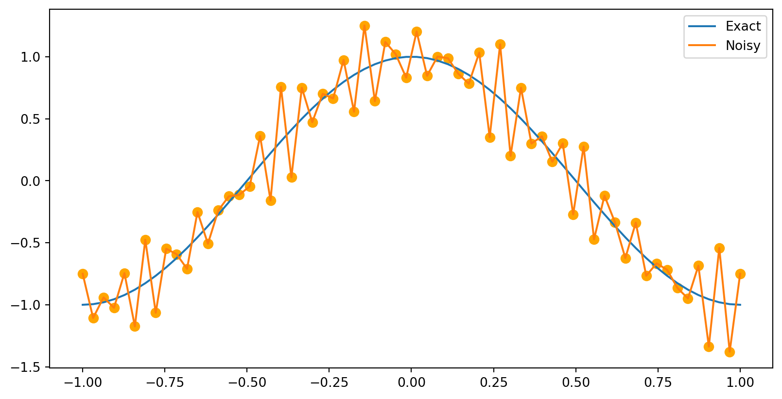
Example: Cleaning up a noisy signal
True signal: \(f(t)=\cos (\pi t),-1 \leq t \leq 1\)
Signal plus noise: \(g(t)=\cos (\pi t)+\) \(\frac{1}{5} \sin (24 \pi t)+\frac{1}{4} \cos (30 \pi t)\)
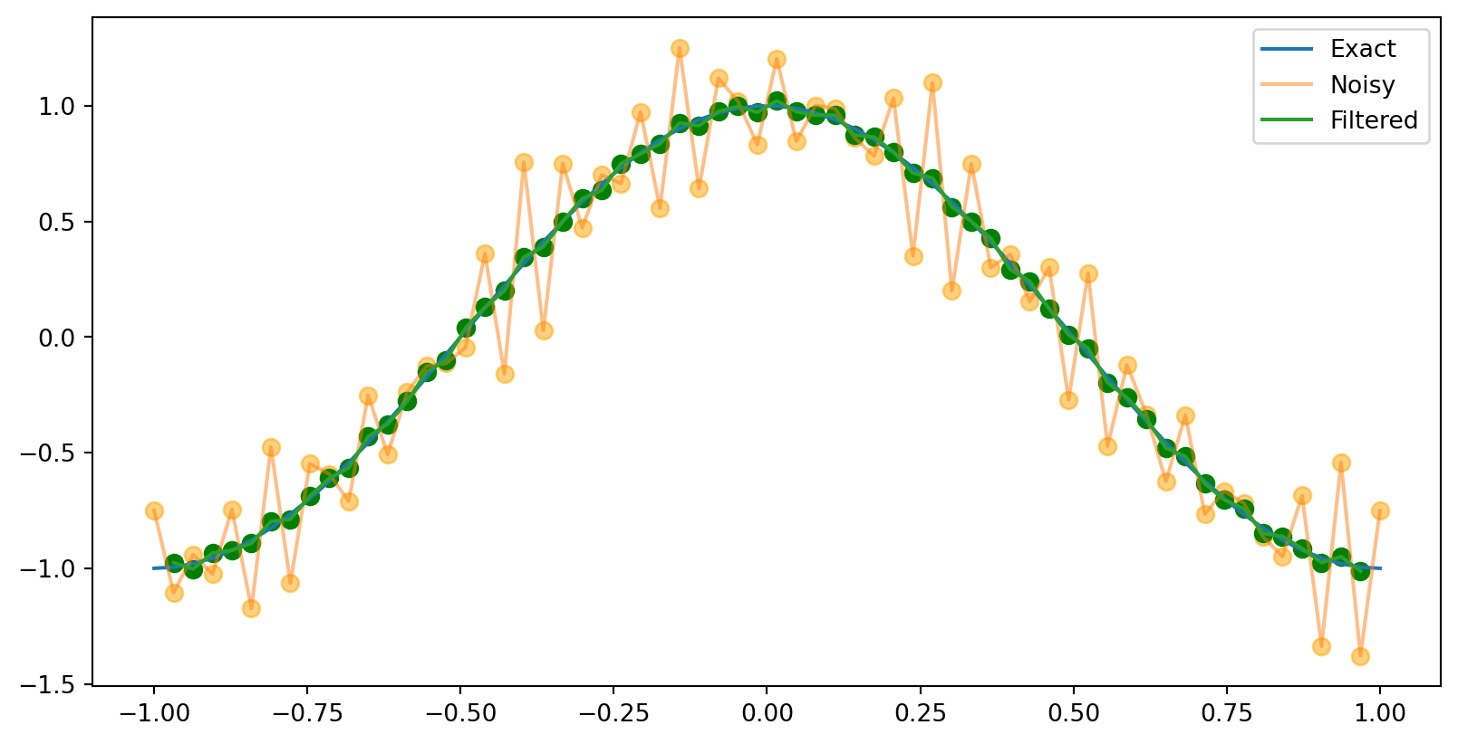
Filtered data
Idea: we can sample nearby points and take a weighted average of them.
\[ y_{k}=\frac{1}{4} x_{k+1}+\frac{1}{2} x_{k}+\frac{1}{4} x_{k-1}, \quad k=1,2, \ldots, 63 \]
. . .
. . .
This captured the low-frequency part of the signal, and filtered out the high-frequency noise. That’s just what we wanted! This is called a low-pass filter.
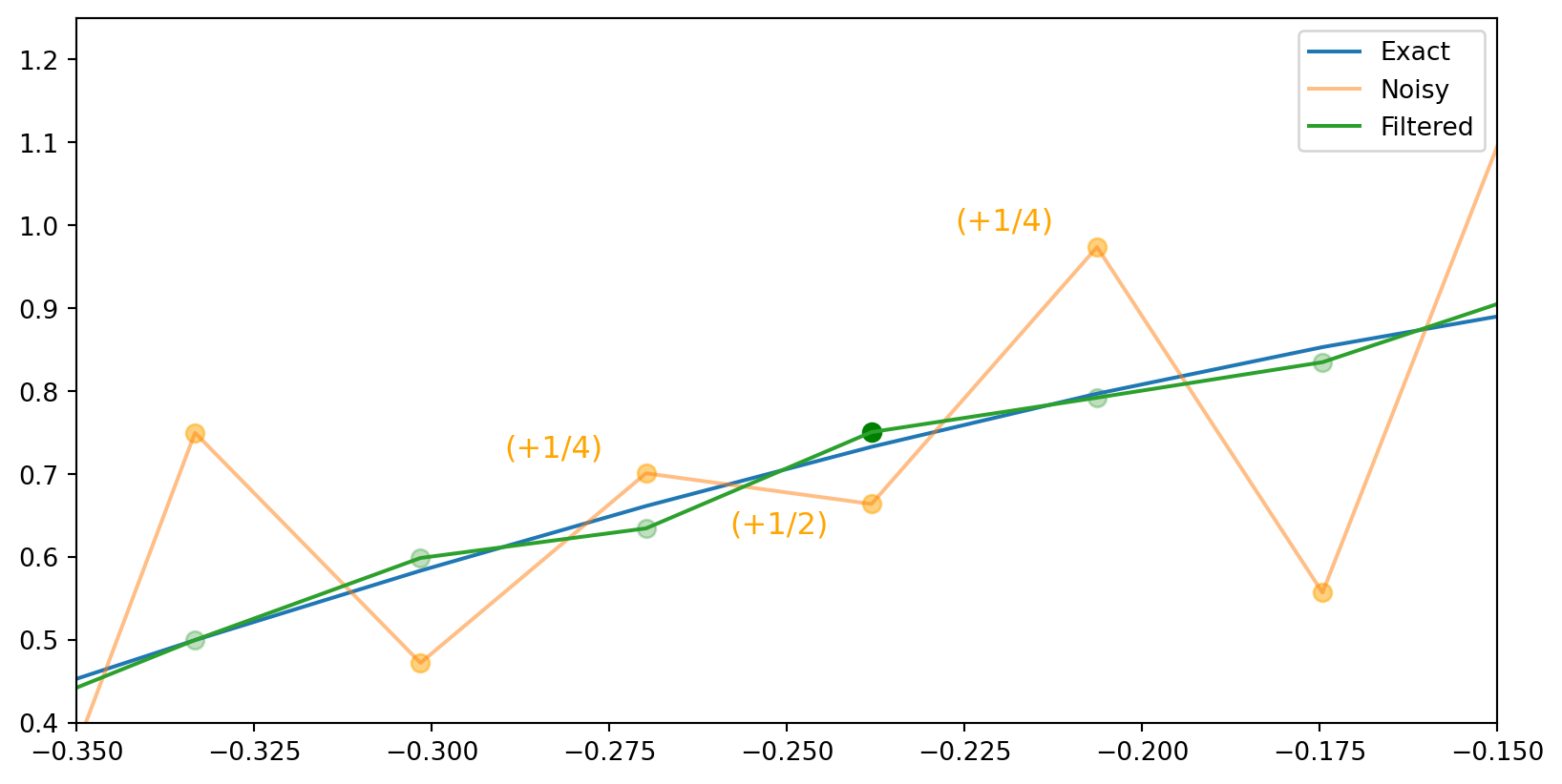
We can zoom in on a few points to see the effect of the filter.
Now you try
See if you can make a figure which will just find the noisyness…
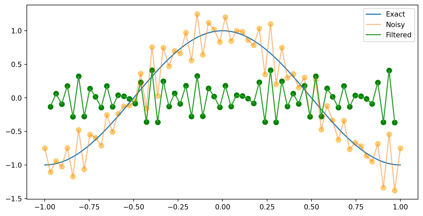
A different filter
What if we subtract the values at \(x_{k+1}\) and \(x_{k-1}\) instead of adding them?
\[ y_{k}=-\frac{1}{4} x_{k+1}+\frac{1}{2} x_{k}-\frac{1}{4} x_{k-1}, \quad k=1,2, \ldots, 63 \]
. . .
. . .
This is a high-pass filter. It captures the high-frequency noise, but filters out the low-frequency signal.
Inverse Matrices
Definition of inverse matrix
Let \(A\) be a square matrix.
Inverse for \(A\) is a square matrix \(B\) of the same size as \(A\)
such that \(A B=I=B A\).
If such a \(B\) exists, then the matrix \(A\) is said to be invertible.
Also called “singular” (non-invertible), or “nonsingular” (invertible)
Conditions for invertibility
Conditions for Invertibility The following are equivalent conditions on the square \(n \times n\) matrix \(A\) :
The matrix \(A\) is invertible.
There is a square matrix \(B\) such that \(B A=I\).
The linear system \(A \mathbf{x}=\mathbf{b}\) has a unique solution for every right-hand-side vector \(\mathbf{b}\).
The linear system \(A \mathbf{x}=\mathbf{b}\) has a unique solution for some right-hand-side vector \(\mathbf{b}\).
The linear system \(A \mathbf{x}=0\) has only the trivial solution.
\(\operatorname{rank} A=n\).
The reduced row echelon form of \(A\) is \(I_{n}\).
The matrix \(A\) is a product of elementary matrices.
There is a square matrix \(B\) such that \(A B=I\).
Elementary matrices
- Each of the operations in row reduction can be represented by a matrix \(E\).
. . .
Remember: - \(E_{i j}\) : The elementary operation of switching the ith and jth rows of the matrix. - \(E_{i}(c)\) : The elementary operation of multiplying the ith row by the nonzero constant \(c\). - \(E_{i j}(d)\) : The elementary operation of adding \(d\) times the jth row to the ith row.
. . .
Find an elementary matrix of size \(n\) is by performing the corresponding elementary row operation on the identity matrix \(I_{n}\).
. . .
Example: Find the elementary matrix for \(E_{13}(-4)\)
. . .
Add -4 times the 3rd row of \(I_{3}\) to its first row…
. . .
\[ E_{13}(-4)=\left[\begin{array}{rrr} 1 & 0 & -4 \\ 0 & 1 & 0 \\ 0 & 0 & 1 \end{array}\right] \]
Recall an example from the first week:
Solve the simple system
\[ \begin{gather*} 2 x-y=1 \\ 4 x+4 y=20 . \tag{1.5} \end{gather*} \]
. . .
\[ \begin{aligned} & {\left[\begin{array}{rrr} 2 & -1 & 1 \\ 4 & 4 & 20 \end{array}\right] \overrightarrow{E_{12}}\left[\begin{array}{rrr} 4 & 4 & 20 \\ 2 & -1 & 1 \end{array}\right] \overrightarrow{E_{1}(1 / 4)}\left[\begin{array}{rrr} 1 & 1 & 5 \\ 2 & -1 & 1 \end{array}\right]} \\ & \overrightarrow{E_{21}(-2)}\left[\begin{array}{rrr} 1 & 1 & 5 \\ 0 & -3 & -9 \end{array}\right] \overrightarrow{E_{2}(-1 / 3)}\left[\begin{array}{lll} 1 & 1 & 5 \\ 0 & 1 & 3 \end{array}\right] \overrightarrow{E_{12}(-1)}\left[\begin{array}{lll} 1 & 0 & 2 \\ 0 & 1 & 3 \end{array}\right] . \end{aligned} \]
Rewrite this using matrix multiplication: \[ \left[\begin{array}{lll} 1 & 0 & 2 \\ 0 & 1 & 3 \end{array}\right]=E_{12}(-1) E_{2}(-1 / 3) E_{21}(-2) E_{1}(1 / 4) E_{12}\left[\begin{array}{rrr} 2 & -1 & 1 \\ 4 & 4 & 20 \end{array}\right] \text {. } \]
Remove the last columns in each matrix above. (They were the “augmented” part of the original problem.) All the operations still work:
\[ \left[\begin{array}{ll} 1 & 0 \\ 0 & 1 \end{array}\right]=E_{12}(-1) E_{2}(-1 / 3) E_{21}(-2) E_{1}(1 / 4) E_{12}\left[\begin{array}{rr} 2 & -1 \\ 4 & 4 \end{array}\right] \text {. } \]
. . .
Aha! We now have a formula for the inverse of the original matrix:
\[ A^{-1}=E_{12}(-1) E_{2}(-1 / 3) E_{21}(-2) E_{1}(1 / 4) E_{12} \]
Superaugmented matrix
Form the superaugmented matrix \([A \mid I]\).
If we perform the elementary operation \(E\) on the superaugmented matrix, we get the matrix \(E\) in the augmented part:
\[ E[A \mid I]=[E A \mid E I]=[E A \mid E] \]
This can help us keep track of our operations as we do row reduction
The augmented part is just the product of the elementary matrices that we have used so far.
Now continue applying elementary row operations until the part of the matrix originally occupied by \(A\) is reduced to the reduced row echelon form of \(A\). . . . \[ [A \mid I] \overrightarrow{E_{1}, E_{2}, \ldots, E_{k}}[I \mid B] \]
\(B=E_{k} E_{k-1} \cdots E_{1}\) is the product of the various elementary matrices we used.
Inverse Algorithm
Given an \(n \times n\) matrix \(A\), to compute \(A^{-1}\) :
Form the superaugmented matrix \(\widetilde{A}=\left[A \mid I_{n}\right]\).
Reduce the first \(n\) columns of \(\tilde{A}\) to reduced row echelon form by performing elementary operations on the matrix \(\widetilde{A}\) resulting in the matrix \([R \mid B]\).
If \(R=I_{n}\) then set \(A^{-1}=B\); otherwise, \(A\) is singular and \(A^{-1}\) does not exist.
2x2 matrices
Suppose we have the 2x2 matrix
\[ A=\left[\begin{array}{ll} a & b \\ c & d \end{array}\right] \]
. . .
Do row reduction on the superaugmented matrix:
\[ \left[\begin{array}{ll|ll} a & b & 1 & 0 \\ c & d & 0 & 1 \end{array}\right] \]
. . .
\[ A^{-1}=\frac{1}{D}\left[\begin{array}{rr} d & -b \\ -c & a \end{array}\right] \]
PageRank revisited
Back to PageRank

Do page ranking as in the first week:
- for page \(j\) let \(n_{j}\) be its total number of outgoing links on that page.
- Then the score for vertex \(i\) is the sum of the scores of all vertices \(j\) that link to \(i\), divided by the total number of outgoing links on page \(j\). . . . \[ \begin{equation*} x_{i}=\sum_{x_{j} \in L_{i}} \frac{x_{j}}{n_{j}} . \tag{1.4} \end{equation*} \]
. . .
\[ \begin{aligned} & x_{1}=\frac{x_{3}}{3} \\ & x_{2}=\frac{x_{1}}{2}+\frac{x_{3}}{3} \\ & x_{3}=\frac{x_{1}}{2}+\frac{x_{2}}{1} \\ & x_{4}=\frac{x_{3}}{3} \\ & x_{5}=\frac{x_{6}}{1} \\ & x_{6}=\frac{x_{5}}{1} \end{aligned} \]
PageRank as a matrix equation
Define the matrix \(Q\) and vector \(\mathbf{x}\) by
\[ Q=\left[\begin{array}{llllll} 0 & 0 & \frac{1}{3} & 0 & 0 & 0 \\ \frac{1}{2} & 0 & \frac{1}{3} & 0 & 0 & 0 \\ \frac{1}{2} & 1 & 0 & 0 & 0 & 0 \\ 0 & 0 & \frac{1}{3} & 0 & 0 & 0 \\ 0 & 0 & 0 & 0 & 0 & 1 \\ 0 & 0 & 0 & 0 & 1 & 0 \end{array}\right], \mathbf{x}=\left(x_{1}, x_{2}, x_{3}, x_{4}, x_{5}\right) \]
. . .
Then the equation \(x=Q x\) is equivalent to the system of equations above.
. . .
\(\mathbf{x}\) is a stationary vector for the transition matrix \(Q\).
Connection between adjacency matrix and transition matrix
- \(A\): adjacency matrix of a graph or digraph
- \(D\): be a diagonal matrix whose \(i\) th entry is either:
- the inverse of the sum of all entries in the \(i\) th row of \(\mathrm{A}\), or
- zero if if this sum is zero.
- Then \(Q=A^{T} D\) is the transition matrix for the page ranking of this graph.
. . . Check:
\[ A=\left[\begin{array}{llllll} 0 & 1 & 1 & 0 & 0 & 0 \\ 0 & 0 & 1 & 0 & 0 & 0 \\ 1 & 1 & 0 & 1 & 0 & 0 \\ 0 & 0 & 0 & 0 & 0 & 0 \\ 0 & 0 & 0 & 0 & 0 & 1 \\ 0 & 0 & 0 & 0 & 1 & 0 \end{array}\right] \]
PageRank as a Markov chain
Think of web surfing as a random process
- each page is a state
- probabilities of moving from one state to another given by a stochastic transition matrix P.
- equal probability of moving to any of the outgoing links of a page
. . .
\[ P\stackrel{?}{=}\left[\begin{array}{llllll} 0 & 0 & \frac{1}{3} & 0 & 0 & 0 \\ \frac{1}{2} & 0 & \frac{1}{3} & 0 & 0 & 0 \\ \frac{1}{2} & 1 & 0 & 0 & 0 & 0 \\ 0 & 0 & \frac{1}{3} & 0 & 0 & 0 \\ 0 & 0 & 0 & 0 & 0 & 1 \\ 0 & 0 & 0 & 0 & 1 & 0 \end{array}\right] \]
Pause: Is \(P\) a stochastic matrix?
Correction vector
We can introduce a correction vector, equivalent to adding links from the dangling node to every other node, or to all connecting nodes (via some path).
. . .
\[ P=\left[\begin{array}{llllll} 0 & 0 & \frac{1}{3} & \frac{1}{3} & 0 & 0 \\ \frac{1}{2} & 0 & \frac{1}{3} & \frac{1}{3} & 0 & 0 \\ \frac{1}{2} & 1 & 0 & \frac{1}{3} & 0 & 0 \\ 0 & 0 & \frac{1}{3} & 0 & 0 & 0 \\ 0 & 0 & 0 & 0 & 0 & 1 \\ 0 & 0 & 0 & 0 & 1 & 0 \end{array}\right] \]
. . .
This is now a stochastic matrix “surfing matrix”
. . .
Find the new transition matrix \(Q\)…
Teleportation
There may not be a single stationary vector for the surfing matrix \(P\).
. . .
Solution: Jump around. Every so often, instead of following a link, jump to a random page.
. . .
How can we modify the surfing matrix to include this?
Introduce a teleportation matrix \(E\), which is a transition matrix that allows the surfer to jump to any page with equal probability.
Pause: What must \(E\) be?
. . .
- Let \(\mathbf{v}\) be the teleportation vector with entries 1/n -Let \(\mathbf{e}=\) \((1,1, \ldots, 1)\) be the vector of all ones.
- Then \(\mathbf{v e}^{T}\) is a stochastic matrix whose columns are all equal to \(\mathbf{v}\). This is \(E\).
PageRank Matrix
Let:
- \(P\) be a stochastic matrix,
- \(\mathbf{v}\) a distribution vector of compatible size
- \(\alpha\) a teleportation parameter with \(0<\alpha<1\).
- Then \(\alpha P+(1-\alpha) \mathbf{v e}^{T}\) and
- . . . our goal is to find stationary vectors \[ \begin{equation*} \left(\alpha P+(1-\alpha) \mathbf{v e}^{T}\right) \mathbf{x}=\mathbf{x} \tag{2.4} \end{equation*} \]
. . .
Rearranging,
\[ \begin{equation*} (I-\alpha P) \mathbf{x}=(1-\alpha) \mathbf{v} \tag{2.5} \end{equation*} \]
Now solve pagerank for our example
Use M.solve(b)…