import sympy as sp
B = sp.Matrix([[2,2,3],[2,4,1],[3,1,2]])/2
x = sp.Matrix(sp.symbols(['x','y','z']))
(x.T*B*x).expand()
\(\displaystyle \left[\begin{matrix}x^{2} + 2 x y + 3 x z + 2 y^{2} + y z + z^{2}\end{matrix}\right]\)
A matrix \(A\) is called positive definite if \(x^{T} A x>0\) for all nonzero vectors \(x\).
. . .
A symmetric matrix \(K=K^{T}\) is positive definite if and only if all of its eigenvalues are strictly positive.
. . .
Proof: If \(\mathbf{x}=\mathbf{v} \neq \mathbf{0}\) is an eigenvector with (necessarily real) eigenvalue \(\lambda\), then
\[ \begin{equation*} 0<\mathbf{v}^{T} K \mathbf{v}=\mathbf{v}^{T}(\lambda \mathbf{v})=\lambda \mathbf{v}^{T} \mathbf{v}=\lambda\|\mathbf{v}\|^{2} \end{equation*} \]
So \(\lambda>0\)
. . .
Conversely, suppose \(K\) has all positive eigenvalues.
Let \(\mathbf{u}_{1}, \ldots, \mathbf{u}_{n}\) be the orthonormal eigenvector basis with \(K \mathbf{u}_{j}=\lambda_{j} \mathbf{u}_{j}\) with \(\lambda_{j}>0\).
\[ \mathbf{x}=c_{1} \mathbf{u}_{1}+\cdots+c_{n} \mathbf{u}_{n}, \quad \text { we obtain } \quad K \mathbf{x}=c_{1} \lambda_{1} \mathbf{u}_{1}+\cdots+c_{n} \lambda_{n} \mathbf{u}_{n} \]
. . .
Therefore,
\[ \mathbf{x}^{T} K \mathbf{x}=\left(c_{1} \mathbf{u}_{1}^{T}+\cdots+c_{n} \mathbf{u}_{n}^{T}\right)\left(c_{1} \lambda_{1} \mathbf{u}_{1}+\cdots+c_{n} \lambda_{n} \mathbf{u}_{n}\right)=\lambda_{1} c_{1}^{2}+\cdots+\lambda_{n} c_{n}^{2}>0 \]
Let \(A=A^{T}\) be a real symmetric \(n \times n\) matrix. Then
. . .
. . .
\[ A=\left(\begin{array}{ll}3 & 1 \\ 1 & 3\end{array}\right) \]
. . .
We compute the determinant in the characteristic equation
\[ \operatorname{det}(A-\lambda \mathrm{I})=\operatorname{det}\left(\begin{array}{cc} 3-\lambda & 1 \\ 1 & 3-\lambda \end{array}\right)=(3-\lambda)^{2}-1=\lambda^{2}-6 \lambda+8 \]
. . .
\[ \lambda^{2}-6 \lambda+8=(\lambda-4)(\lambda-2)=0 \]
. . .
Eigenvectors:
For the first eigenvalue, the eigenvector equation is
\[ (A-4 \mathrm{I}) \mathbf{v}=\left(\begin{array}{rr} -1 & 1 \\ 1 & -1 \end{array}\right)\binom{x}{y}=\binom{0}{0}, \quad \text { or } \quad \begin{array}{r} -x+y=0 \\ x-y=0 \end{array} \]
General solution: \[ x=y=a, \quad \text { so } \quad \mathbf{v}=\binom{a}{a}=a\binom{1}{1} \]
. . . \[ \lambda_{1}=4, \quad \mathbf{v}_{1}=\binom{1}{1}, \quad \lambda_{2}=2, \quad \mathbf{v}_{2}=\binom{-1}{1} \]
. . .
The eigenvectors are orthogonal: \(\mathbf{v}_{1} \cdot \mathbf{v}_{2}=0\)
Let \(A=A^{T}\) be a real symmetric \(n \times n\) matrix. Then
. . .
Suppose \(\lambda\) is a complex eigenvalue with complex eigenvector \(\mathbf{v} \in \mathbb{C}^{n}\).
\[ (A \mathbf{v}) \cdot \mathbf{v}=(\lambda \mathbf{v}) \cdot \mathbf{v}=\lambda\|\mathbf{v}\|^{2} \]
. . .
Now, if \(A\) is real and symmetric,
\[ \begin{equation*} (A \mathbf{v}) \cdot \mathbf{w}=\left(\mathbf{v}^T A^T \right)\mathbf{w} = \mathbf{v} \cdot(A \mathbf{w}) \quad \text { for all } \quad \mathbf{v}, \mathbf{w} \in \mathbb{C}^{n} \end{equation*} \]
Therefore
\[ (A \mathbf{v}) \cdot \mathbf{v}=\mathbf{v} \cdot(A \mathbf{v})=\mathbf{v} \cdot(\lambda \mathbf{v})=\mathbf{v}^{T} \overline{\lambda \mathbf{v}}=\bar{\lambda}\|\mathbf{v}\|^{2} \]
. . .
\(\Rightarrow\), \(\lambda\|\mathbf{v}\|^{2}=\bar{\lambda}\|\mathbf{v}\|^{2}\) \(\Rightarrow\) \(\lambda=\bar{\lambda}\), so \(\lambda\) is real.
Part b: Eigenvectors corresponding to distinct eigenvalues are orthogonal.
Suppose \(A \mathbf{v}=\lambda \mathbf{v}, A \mathbf{w}=\mu \mathbf{w}\), where \(\lambda \neq \mu\) are distinct real eigenvalues.
. . .
\(\lambda \mathbf{v} \cdot \mathbf{w}=(A \mathbf{v}) \cdot \mathbf{w}=\mathbf{v} \cdot(A \mathbf{w})=\mathbf{v} \cdot(\mu \mathbf{w})=\mu \mathbf{v} \cdot \mathbf{w}, \quad\) and hence \(\quad(\lambda-\mu) \mathbf{v} \cdot \mathbf{w}=0\).
. . .
Since \(\lambda \neq \mu\), this implies that \(\mathbf{v} \cdot \mathbf{w}=0\), so the eigenvectors \(\mathbf{v}, \mathbf{w}\) are orthogonal.
Part c: There is an orthonormal basis of \(\mathbb{R}^{n}\) consisting of \(n\) eigenvectors of \(A\).
. . .
If the eigenvalues are distinct, then the eigenvectors are orthogonal by part (b).
. . .
If the eigenvalues are repeated, then we can use the Gram-Schmidt process to orthogonalize the eigenvectors.
. . .
Writing our diagonalization from the previous lecture, specifically for the case of a real symmetric matrix \(A\):
If \(A=A^{T}\) is a real symmetric \(n \times n\) matrix, then there exists an orthogonal matrix \(Q\) and a real diagonal matrix \(\Lambda\) such that
\[ \begin{equation*} A=Q \Lambda Q^{-1}=Q \Lambda Q^{T} \end{equation*} \]
The eigenvalues of \(A\) appear on the diagonal of \(\Lambda\), while the columns of \(Q\) are the corresponding orthonormal eigenvectors.
A quadratic form is a homogeneous polynomial of degree 2 in \(n\) variables \(x_{1}, \ldots, x_{n}\). For example, in \(x, y, z\): \(Q(x, y, z)=a x^{2}+b y^{2}+c z^{2}+2 d x y+2 e y z+2 f z x\).
. . .
Every quadratic form can be written in matrix form as \(Q(\mathbf{x})=\mathbf{x}^{T} A \mathbf{x}\).
. . .
Example:
\[ Q(x, y, z)=x^{2}+2 y^{2}+z^{2}+2 x y+y z+3 x z . \]
. . .
\[ \begin{aligned} x(x+2 y+3 z)+y(2 y+z)+z^{2} & =\left[\begin{array}{lll} x & y & z \end{array}\right]\left[\begin{array}{c} x+2 y+3 z \\ 2 y+z \\ z \end{array}\right] \\ & =\left[\begin{array}{lll} x & y & z \end{array}\right]\left[\begin{array}{lll} 1 & 2 & 3 \\ 0 & 2 & 1 \\ 0 & 0 & 1 \end{array}\right]\left[\begin{array}{c} x \\ y \\ z \end{array}\right]=\mathbf{x}^{T} A \mathbf{x}, \end{aligned} \]
Now, if we have a quadratic form \(Q(\mathbf{x})=\mathbf{x}^{T} A \mathbf{x}\), we always write this in terms of an equivalent symmetric matrix \(B\) as \(Q(\mathbf{x})=\mathbf{x}^{T} B \mathbf{x}\) where \(B=\frac{1}{2}(A+A^{T})\).
(See Exercise 2.4.34 in your texbook.)
So in this case, we can write \(Q(\mathbf{x})=\mathbf{x}^{T} B \mathbf{x}\) where
\[ B=\frac{1}{2}\left[\begin{array}{lll} 2 & 2 & 3 \\ 2 & 4 & 1 \\ 3 & 1 & 2 \end{array}\right] \]
Check:
import sympy as sp
B = sp.Matrix([[2,2,3],[2,4,1],[3,1,2]])/2
x = sp.Matrix(sp.symbols(['x','y','z']))
(x.T*B*x).expand()\(\displaystyle \left[\begin{matrix}x^{2} + 2 x y + 3 x z + 2 y^{2} + y z + z^{2}\end{matrix}\right]\)
Yes, this is the same as the original quadratic form.
Symmetric matrices are diagonalizable \(\Rightarrow\) we can always find a basis in which the quadratic form takes a particularly simple form. Just diagonalize:
. . .
\(Q(\mathbf{x})=\mathbf{x}^{T} B \mathbf{x}=x^{T} P D P^{T} x\) where \(P\) is the matrix of eigenvectors of \(B\) and \(D\) is the diagonal matrix of eigenvalues of \(B\).
. . .
Then if we define new variables \(\mathbf{y}=P^{T} \mathbf{x}\), we have \(Q(\mathbf{x})=\mathbf{y}^{T} D \mathbf{y}\)
. . .
which just becomes a sum of squares:
\[ q(\mathbf{x})=\lambda_{1} y_{1}^{2}+\cdots+\lambda_{n} y_{n}^{2} \]
Example:
Suppose we have the quadratic form \(3x^2+2xy+3y^2\). We can write this in matrix form as \(Q(\mathbf{x})=\mathbf{x}^{T} B \mathbf{x}\) where \(\mathbf{x}=\binom{x_1}{x_2}\) and
\[ B=\frac{1}{2}\left[\begin{array}{ll} 3 & 1 \\ 1 & 3 \end{array}\right] \]
. . .
We diagonalize \(B\):
\[ \left(\begin{array}{ll} 3 & 1 \\ 1 & 3 \end{array}\right)=A=P D P^{T}=\left(\begin{array}{cc} \frac{1}{\sqrt{2}} & -\frac{1}{\sqrt{2}} \\ \frac{1}{\sqrt{2}} & \frac{1}{\sqrt{2}} \end{array}\right)\left(\begin{array}{ll} 4 & 0 \\ 0 & 2 \end{array}\right)\left(\begin{array}{cc} \frac{1}{\sqrt{2}} & \frac{1}{\sqrt{2}} \\ -\frac{1}{\sqrt{2}} & \frac{1}{\sqrt{2}} \end{array}\right) \]
. . .
Now, if we define \(\mathbf{y}=P^{T} \mathbf{x}=\frac{1}{\sqrt{2}}\binom{x_1+x_2}{-x_1+x_2}\), we have \(Q(\mathbf{x})=\mathbf{y}^{T} D \mathbf{y}\), or
\[ q(\mathbf{x})=3 x_{1}^{2}+2 x_{1} x_{2}+3 x_{2}^{2}=4 y_{1}^{2}+2 y_{2}^{2} \]
The numbers aren’t always clean, though!
Q,Lambda = B.diagonalize()
Q
\(\displaystyle \left[\begin{matrix}\frac{- 13248 \cdot \left(1 + \sqrt{3} i\right) \left(53 + 9 \sqrt{1167} i\right)^{\frac{2}{3}} - \sqrt[3]{53 + 9 \sqrt{1167} i} \left(184 + \left(-16 + \left(1 + \sqrt{3} i\right) \sqrt[3]{53 + 9 \sqrt{1167} i}\right) \left(1 + \sqrt{3} i\right) \sqrt[3]{53 + 9 \sqrt{1167} i}\right)^{2} + 72 \left(1 + \sqrt{3} i\right)^{2} \cdot \left(11 - \left(1 + \sqrt{3} i\right) \sqrt[3]{53 + 9 \sqrt{1167} i}\right) \left(53 + 9 \sqrt{1167} i\right)}{792 \left(1 + \sqrt{3} i\right)^{2} \cdot \left(53 + 9 \sqrt{1167} i\right)} & \frac{72 \left(1 - \sqrt{3} i\right)^{3} \cdot \left(11 + \left(-1 + \sqrt{3} i\right) \sqrt[3]{53 + 9 \sqrt{1167} i}\right) \left(53 + 9 \sqrt{1167} i\right) + \left(-1 + \sqrt{3} i\right) \sqrt[3]{53 + 9 \sqrt{1167} i} \left(184 + \left(-16 + \left(1 - \sqrt{3} i\right) \sqrt[3]{53 + 9 \sqrt{1167} i}\right) \left(1 - \sqrt{3} i\right) \sqrt[3]{53 + 9 \sqrt{1167} i}\right)^{2} - 13248 \left(1 - \sqrt{3} i\right)^{2} \left(53 + 9 \sqrt{1167} i\right)^{\frac{2}{3}}}{792 \left(1 - \sqrt{3} i\right)^{3} \cdot \left(53 + 9 \sqrt{1167} i\right)} & \frac{126 \sqrt{1167} - 289 i \left(53 + 9 \sqrt{1167} i\right)^{\frac{2}{3}} - 3 \sqrt{1167} \left(53 + 9 \sqrt{1167} i\right)^{\frac{2}{3}} - 742 i + 352 i \sqrt[3]{53 + 9 \sqrt{1167} i} + 60 \sqrt{1167} \sqrt[3]{53 + 9 \sqrt{1167} i}}{66 \cdot \left(9 \sqrt{1167} - 53 i\right)}\\\frac{28 \left(-22 + \left(1 + \sqrt{3} i\right) \sqrt[3]{53 + 9 \sqrt{1167} i}\right) \left(1 + \sqrt{3} i\right)^{2} \cdot \left(53 + 9 \sqrt{1167} i\right) + \sqrt[3]{53 + 9 \sqrt{1167} i} \left(184 + \left(-16 + \left(1 + \sqrt{3} i\right) \sqrt[3]{53 + 9 \sqrt{1167} i}\right) \left(1 + \sqrt{3} i\right) \sqrt[3]{53 + 9 \sqrt{1167} i}\right)^{2} + 5152 \cdot \left(1 + \sqrt{3} i\right) \left(53 + 9 \sqrt{1167} i\right)^{\frac{2}{3}}}{264 \left(1 + \sqrt{3} i\right)^{2} \cdot \left(53 + 9 \sqrt{1167} i\right)} & \frac{5152 \cdot \left(1 - \sqrt{3} i\right) \left(53 + 9 \sqrt{1167} i\right)^{\frac{2}{3}} + \sqrt[3]{53 + 9 \sqrt{1167} i} \left(184 + \left(-16 + \left(1 - \sqrt{3} i\right) \sqrt[3]{53 + 9 \sqrt{1167} i}\right) \left(1 - \sqrt{3} i\right) \sqrt[3]{53 + 9 \sqrt{1167} i}\right)^{2} + 28 \left(-22 + \left(1 - \sqrt{3} i\right) \sqrt[3]{53 + 9 \sqrt{1167} i}\right) \left(1 - \sqrt{3} i\right)^{2} \cdot \left(53 + 9 \sqrt{1167} i\right)}{264 \left(1 - \sqrt{3} i\right)^{2} \cdot \left(53 + 9 \sqrt{1167} i\right)} & \frac{18 \sqrt{1167} - 2222 i \sqrt[3]{53 + 9 \sqrt{1167} i} - 145 i \left(53 + 9 \sqrt{1167} i\right)^{\frac{2}{3}} - 106 i + 18 \sqrt{1167} \sqrt[3]{53 + 9 \sqrt{1167} i} + 9 \sqrt{1167} \left(53 + 9 \sqrt{1167} i\right)^{\frac{2}{3}}}{66 \cdot \left(9 \sqrt{1167} - 53 i\right)}\\1 & 1 & 1\end{matrix}\right]\)
Lambda\(\displaystyle \left[\begin{matrix}\frac{4}{3} + \left(- \frac{1}{2} - \frac{\sqrt{3} i}{2}\right) \sqrt[3]{\frac{53}{216} + \frac{\sqrt{1167} i}{24}} + \frac{23}{18 \left(- \frac{1}{2} - \frac{\sqrt{3} i}{2}\right) \sqrt[3]{\frac{53}{216} + \frac{\sqrt{1167} i}{24}}} & 0 & 0\\0 & \frac{4}{3} + \frac{23}{18 \left(- \frac{1}{2} + \frac{\sqrt{3} i}{2}\right) \sqrt[3]{\frac{53}{216} + \frac{\sqrt{1167} i}{24}}} + \left(- \frac{1}{2} + \frac{\sqrt{3} i}{2}\right) \sqrt[3]{\frac{53}{216} + \frac{\sqrt{1167} i}{24}} & 0\\0 & 0 & \frac{4}{3} + \frac{23}{18 \sqrt[3]{\frac{53}{216} + \frac{\sqrt{1167} i}{24}}} + \sqrt[3]{\frac{53}{216} + \frac{\sqrt{1167} i}{24}}\end{matrix}\right]\)
Yuck!
We can visualize the previous example as a rotation of the axes (a change of basis) to a new coordinate system where the quadratic form is just a sum of squares.
import numpy as np
import matplotlib.pyplot as plt
x = np.linspace(-2,2,100)
y = np.linspace(-2,2,100)
X,Y = np.meshgrid(x,y)
Z = 3*X**2+2*X*Y+3*Y**2
plt.contour(X,Y,Z,levels=[1,2,3,4,5,6,7,8,9,10])
plt.xlabel('x1')
plt.ylabel('x2')
plt.axis('equal')
# plot the vector P.T times (1,0) and (0,1)
P = np.array([[1/np.sqrt(2),1/np.sqrt(2)],[-1/np.sqrt(2),1/np.sqrt(2)]])
v1 = P.T @ np.array([1,0])
v2 = P.T @ np.array([0,1])
plt.quiver(0,0,v1[0],v1[1],angles='xy',scale_units='xy',scale=1,color='r')
plt.quiver(0,0,v2[0],v2[1],angles='xy',scale_units='xy',scale=1,color='r')
# label the two quivers ("x1=1, x2=0" and "x1=0, x2=1")
plt.text(v1[0],v1[1],'y(x1=1,x2=0)',fontsize=12)
plt.text(v2[0],v2[1],'y(x1=0,x2=1)',fontsize=12)
plt.show()
Now make the same plot but in y coordinates:
x = np.linspace(-2,2,100)
y = np.linspace(-2,2,100)
X,Y = np.meshgrid(x,y)
Z = 4*X**2+2*Y**2
plt.contour(X,Y,Z,levels=[1,2,3,4,5,6,7,8,9,10])
plt.xlabel('y1')
plt.ylabel('y2')
plt.axis('equal')
v1 = P.T @ np.array([1,0])
v2 = P.T @ np.array([0,1])
plt.quiver(0,0,1,0,angles='xy',scale_units='xy',scale=1,color='r')
plt.quiver(0,0,0,1,angles='xy',scale_units='xy',scale=1,color='r')
# label the two quivers ("x1=1, x2=0" and "x1=0, x2=1")
plt.show()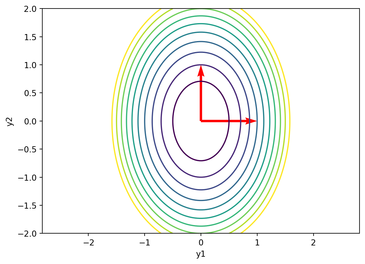
In general, we can think of the diagonalization as a rotation of the axes followed by a scaling of the axes.
We often visualize this by plotting the effects of the transformations on the unit circle.

We’ve talked a lot about eigenvalues and eigenvectors, but these only make any sense for square matrices. What can we do for a general \(m \times n\) matrix \(A\)?
. . .
It turns out we can learn a lot from the matrix \(A^{T} A\) (or \(A A^{T}\)), which is always square and symmetric.
. . .
The singular values \(\sigma_{1}, \ldots, \sigma_{r}\) of an \(m \times n\) matrix \(A\) are the positive square roots, \(\sigma_{i}=\sqrt{\lambda_{i}}>0\), of the nonzero eigenvalues of the associated “Gram matrix” \(K=A^{T} A\).
. . .
The corresponding eigenvectors of \(K\) are known as the singular vectors of \(A\).
. . .
All of the eigenvalues of \(K\) are real and nonnegative – but some may be zero.
. . .
If \(K=A^{T} A\) has repeated eigenvalues, the singular values of \(A\) are repeated with the same multiplicities.
. . .
The number \(r\) of singular values is equal to the rank of the matrices \(A\) and \(K\).
Let \(A=\left(\begin{array}{ll}3 & 5 \\ 4 & 0\end{array}\right)\).
\[ K=A^{T} A=\left(\begin{array}{ll} 3 & 4 \\ 5 & 0 \end{array}\right)\left(\begin{array}{ll} 3 & 5 \\ 4 & 0 \end{array}\right)=\left(\begin{array}{ll} 25 & 15 \\ 15 & 25 \end{array}\right) \]
. . .
This has eigenvalues \(\lambda_{1}=40, \lambda_{2}=10\), and corresponding eigenvectors \(\mathbf{v}_{1}=\binom{1}{1}, \mathbf{v}_{2}=\binom{1}{-1}\).
. . .
Therefore, the singular values of \(A\) are \(\sigma_{1}=\sqrt{40}=2 \sqrt{10}, \sigma_{2}=\sqrt{10}\).
pause
Let \(A\) be an \(m \times n\) real matrix. Then there exist an \(m \times m\) orthogonal matrix \(U\), an \(n \times n\) orthogonal matrix \(V\), and an \(m \times n\) diagonal matrix \(\Sigma\) with diagonal entries \(\sigma_{1} \geq \sigma_{2} \geq \cdots \geq \sigma_{p} \geq 0\), with \(p=\min \{m, n\}\), such that \(U^{T} A V=\Sigma\). Moreover, the numbers \(\sigma_{1}, \sigma_{2}, \ldots, \sigma_{p}\) are uniquely determined by \(A\).
Proof:
(following closely this blog post)
Goal: to understand the SVD as finding perpendicular axes that remain perpendicular after a transformation.

Take a very simple matrix:
\[ A=\left(\begin{array}{cc} 6 & 2 \\ -7 & 6 \end{array}\right) \]
. . .
Represents a linear map \(\mathrm{T}: \mathrm{R}^{2} \rightarrow \mathbf{R}^{2}\) with respect to the standard basis \(e_{1}=(1,0)\) and \(e_{2}=(0,1)\).
. . .
Sends the usual basis elements \(e_{1} \rightsquigarrow(6,-7)\) and \(e_{2} \rightsquigarrow(2,6)\).
We can see what T does to any vector:
\[ \begin{aligned} T(2,3) & =T(2,0)+T(0,3)=T\left(2 e_{1}\right)+T\left(3 e_{2}\right) \\ & =2 T\left(e_{1}\right)+3 T\left(e_{2}\right)=2(6,-7)+3(2,6) \\ & =(18,4) \end{aligned} \]
The usual basis elements are no longer perpendicular after the transformation:

Given a linear map T:Rm \(\rightarrow R^{n}\) (which is represented by a \(n \times m\) matrix \(A\) with respect to the standard basis),
. . .
This is what the SVD does!
Let the SVD of \(A\) be \(A=U \Sigma V^{T}\)
. . .

How are \(U\) and \(V\) related?