[[-0.57294952 -0.81959066]
 [ 0.81959066 -0.57294952]]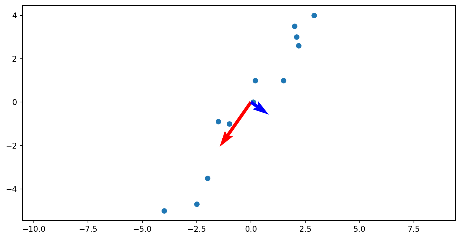
Many parts of this inspired by this blog post
\[ A=U S V^{T} \]
where
$$ \[\begin{array}{lccc} & & & U & V & S \\ & & &\left(\begin{array}{ccc} \mid & & \mid \\ \mathbf{u}_{1} & \cdots & \mathbf{u}_{m} \\ \mid & & \mid \end{array}\right) &\left(\begin{array}{ccc} \mid & & \mid \\ \mathbf{v}_{1} & \cdots & \mathbf{v}_{n} \\ \mid & & \mid \end{array}\right) &\left(\begin{array}{cccc} \sigma_1 & & & \\ & \sigma_2 & \\ & & \ddots & \\ & & & \sigma_r & \\ & & & & \ddots \\ & & & & & 0 \end{array}\right)\\ \text{eigenvectors of} & & & A A^{T} & A^{T} A \\ \end{array}\]$$
\[ A=\left(\begin{array}{ccc} 3 & 2 & 2 \\ 2 & 3 & -2 \end{array}\right) \]
. . .
\[ A A^{T}=\left(\begin{array}{cc} 17 & 8 \\ 8 & 17 \end{array}\right), \quad A^{T} A=\left(\begin{array}{ccc} 13 & 12 & 2 \\ 12 & 13 & -2 \\ 2 & -2 & 8 \end{array}\right) \]
\[ \begin{array}{cc} A A^{T}=\left(\begin{array}{cc} 17 & 8 \\ 8 & 17 \end{array}\right) & A^{T} A=\left(\begin{array}{ccc} 13 & 12 & 2 \\ 12 & 13 & -2 \\ 2 & -2 & 8 \end{array}\right) \\ \begin{array}{c} \text { eigenvalues: } \lambda_{1}=25, \lambda_{2}=9 \\ \text { eigenvectors } \end{array} & \begin{array}{c} \text { eigenvalues: } \lambda_{1}=25, \lambda_{2}=9, \lambda_{3}=0 \\ \text { eigenvectors } \end{array} \\ u_{1}=\binom{1 / \sqrt{2}}{1 / \sqrt{2}} \quad u_{2}=\binom{1 / \sqrt{2}}{-1 / \sqrt{2}} & v_{1}=\left(\begin{array}{c} 1 / \sqrt{2} \\ 1 / \sqrt{2} \\ 0 \end{array}\right) \quad v_{2}=\left(\begin{array}{c} 1 / \sqrt{18} \\ -1 / \sqrt{18} \\ 4 / \sqrt{18} \end{array}\right) \quad v_{3}=\left(\begin{array}{c} 2 / 3 \\ -2 / 3 \\ -1 / 3 \end{array}\right) \end{array} \]
SVD decomposition of \(A\): \[ A=U S V^{T}=\left(\begin{array}{cc} 1 / \sqrt{2} & 1 / \sqrt{2} \\ 1 / \sqrt{2} & -1 / \sqrt{2} \end{array}\right)\left(\begin{array}{ccc} 5 & 0 & 0 \\ 0 & 3 & 0 \end{array}\right)\left(\begin{array}{rrr} 1 / \sqrt{2} & 1 / \sqrt{2} & 0 \\ 1 / \sqrt{18} & -1 / \sqrt{18} & 4 / \sqrt{18} \\ 2 / 3 & -2 / 3 & -1 / 3 \end{array}\right) \]
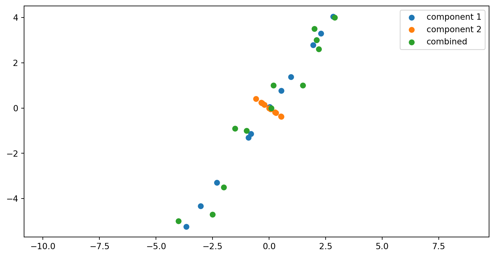
\[ A=\sigma_{l} u_{l} v_{l}^{T}+\ldots+\sigma_{r} u_{r} v_{r}^{T} \]
\[ A=\left(\begin{array}{ccc} 3 & 2 & 2 \\ 2 & 3 & -2 \end{array}\right) \]
. . .
Can decompose as

. . .
\(=\left(\begin{array}{ccc}3 & 2 & 2 \\ 2 & 3 & -2\end{array}\right)\)
If we have a linear system
\[ \begin{aligned} A x & =b \\ \end{aligned} \]
and \(A\) is invertible, then we can solve for \(x\):
\[ \begin{aligned} x & =A^{-1} b \end{aligned} \]
. . .
If \(A\) is not invertible, we can define instead a pseudoinverse \(A^{+}\)
. . .
Define \(A^{+}\) in order to minimize the least squares error:
\[ \left\|\mathbf{A} \mathbf{A}^{+}-\mathbf{I}_{\mathbf{n}}\right\|_{2} \]
. . .
Then we can estimate \(x\) as
\[ \begin{aligned} A x & =b \\ x & \approx A^{+} b \end{aligned} \]
\(A^T=\left[\begin{array}{rrrrrrrrrrrr}2.9 & -1.5 & 0.1 & -1.0 & 2.1 & -4.0 & -2.0 & 2.2 & 0.2 & 2.0 & 1.5 & -2.5 \\ 4.0 & -0.9 & 0.0 & -1.0 & 3.0 & -5.0 & -3.5 & 2.6 & 1.0 & 3.5 & 1.0 & -4.7\end{array}\right]\)
. . .

Covariance: \[ \begin{aligned} \sigma_{a b}^{2} & =\operatorname{cov}(a, b)=\mathrm{E}[(a-\bar{a})(b-\bar{b})] \\ \sigma_{a}^{2} & =\operatorname{var}(a)=\operatorname{cov}(a, a)=\mathrm{E}\left[(a-\bar{a})^{2}\right] \end{aligned} \]
. . .
Covariance matrix:
\[ \mathbf{\Sigma}=\left(\begin{array}{cccc} E\left[\left(x_{1}-\mu_{1}\right)\left(x_{1}-\mu_{1}\right)\right] & E\left[\left(x_{1}-\mu_{1}\right)\left(x_{2}-\mu_{2}\right)\right] & \ldots & E\left[\left(x_{1}-\mu_{1}\right)\left(x_{p}-\mu_{p}\right)\right] \\ E\left[\left(x_{2}-\mu_{2}\right)\left(x_{1}-\mu_{1}\right)\right] & E\left[\left(x_{2}-\mu_{2}\right)\left(x_{2}-\mu_{2}\right)\right] & \ldots & E\left[\left(x_{2}-\mu_{2}\right)\left(x_{p}-\mu_{p}\right)\right] \\ \vdots & \vdots & \ddots & \vdots \\ E\left[\left(x_{p}-\mu_{p}\right)\left(x_{1}-\mu_{1}\right)\right] & E\left[\left(x_{p}-\mu_{p}\right)\left(x_{2}-\mu_{2}\right)\right] & \ldots & E\left[\left(x_{p}-\mu_{p}\right)\left(x_{p}-\mu_{p}\right)\right] \end{array}\right) \]
. . .
\[ \Sigma=\mathrm{E}\left[(X-\bar{X})(X-\bar{X})^{\mathrm{T}}\right] \]
. . . \[ \Sigma=\frac{X X^{\mathrm{T}}}{n} \quad \text { (if } X \text { is already zero centered) } \]
. . .
For our dataset,
\[ \text { Sample covariance } S^{2}=\frac{A^{T} A}{(\mathrm{n}-1)}=\frac{1}{11}\left[\begin{array}{rr} 53.46 & 73.42 \\ 73.42 & 107.16 \end{array}\right] \]
\(A^T=\left[\begin{array}{rrrrrrrrrrrr}2.9 & -1.5 & 0.1 & -1.0 & 2.1 & -4.0 & -2.0 & 2.2 & 0.2 & 2.0 & 1.5 & -2.5 \\ 4.0 & -0.9 & 0.0 & -1.0 & 3.0 & -5.0 & -3.5 & 2.6 & 1.0 & 3.5 & 1.0 & -4.7\end{array}\right]\)
. . .
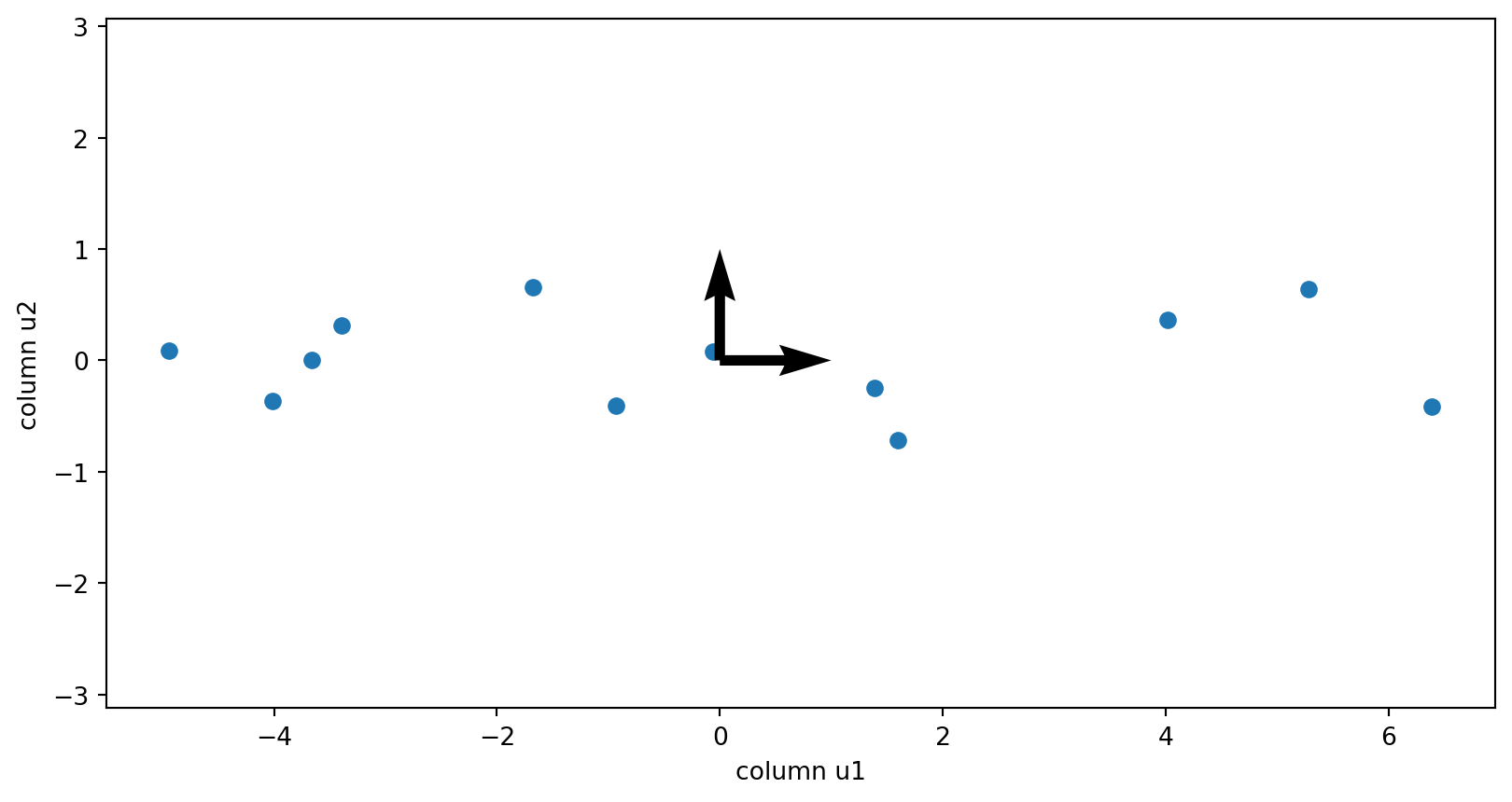
The columns of the V matrix:
[[-0.57294952 -0.81959066]
[ 0.81959066 -0.57294952]]
Walk through why these vectors are actually the eigenvectors of the covariance matrix.
The components of the data matrix
[[4.86       6.67454545]
 [6.67454545 9.74181818]]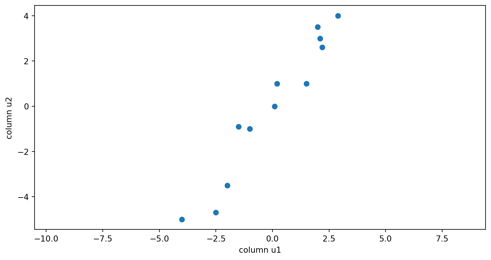
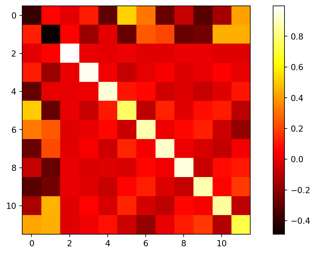
The columns of the U matrix are no longer orthogonal.
The U matrix as a heat plot