More Systems of Linear Equations

Outline for today

• Intuitions about RRE form
• Example + tutorial: Pagerank
• Diffusion
• Reaction-Diffusion in Biology

A resource for review

The glossary from the end of Strand: glossary.pdf

Intuitions about RRE form

Systems with non-unique solutions

Solve for the variables x, y, and z in the system

\begin{aligned} z & =2 \\ x+y+z & =2 \\ 2 x+2 y+4 z & =8 \end{aligned}

Make an augmented matrix:

\left[\begin{array}{llll} 0 & 0 & 1 & 2 \\ 1 & 1 & 1 & 2 \\ 2 & 2 & 4 & 8 \end{array}\right]

Note that the first column corresponds to x, the second to y, and the third to z.

\left[\begin{array}{llll} 0 & 0 & 1 & 2 \\ 1 & 1 & 1 & 2 \\ 2 & 2 & 4 & 8 \end{array}\right] \stackrel{E_{12}}{\longrightarrow}\left[\begin{array}{llll} 1 & 1 & 1 & 2 \\ 0 & 0 & 1 & 2 \\ 2 & 2 & 4 & 8 \end{array}\right] \xrightarrow[E_{31}(-2)]{\longrightarrow}\left[\begin{array}{rlll} 1 & 1 & 1 & 2 \\ 0 & 0 & 2 & 4 \\ 0 & 0 & 1 & 2 \end{array}\right]

Now we are stuck! The first row we are going to use to solve for x. Neither the second or third row tell us anything about y…

We keep on going… \begin{aligned} & {\left[\begin{array}{rrrr} 1 & 1 & 1 & 2 \\ 0 & 0 & 2 & 4 \\ 0 & 0 & 1 & 2 \end{array}\right] \xrightarrow[E_{2}(1 / 2)]{\longrightarrow}\left[\begin{array}{rrrr} 1 & 1 & 1 & 2 \\ 0 & 0 & 1 & 2 \\ 0 & 0 & 1 & 2 \end{array}\right]} \\ & \overrightarrow{E_{32}(-1)}\left[\begin{array}{rrrr} 1 & 1 & 1 & 2 \\ 0 & 0 & 1 & 2 \\ 0 & 0 & 0 & 0 \end{array}\right] \xrightarrow[E_{12}(-1)]{\longrightarrow}\left[\begin{array}{rrrr} 1 & 1 & 0 & 0 \\ 0 & 0 & 1 & 2 \\ 0 & 0 & 0 & 0 \end{array}\right] . \end{aligned}

We have ended up with this matrix:

\left[\begin{array}{rrrr} 1 & 1 & 0 & 0 \\ 0 & 0 & 1 & 2 \\ 0 & 0 & 0 & 0 \end{array}\right]

How can we use this to solve for z? What about x?

But there’s no information on y! It can be anything!!

\begin{aligned} & x=-y \\ & z=2 \\ & y \text { is free. } \end{aligned}

Free versus bound variables

We define a free variable as one that isn’t constrained by the equations. We can assign it any value we want, and the system will still have a solution.

A bound variable is one that is constrained by the equations.

Free versus bound variables in augmented matrices

Suppose we have another augmented matrix, which after GJ elimination has become:

\left[\begin{array}{rrrrr} x & y & z & w & \mathrm{rhs} \\ 1 & 2 & 0 & -1 & 2 \\ 0 & 0 & 1 & 3 & 0 \\ 0 & 0 & 0 & 0 & 0 \end{array}\right] .

The solutions are: \begin{aligned} x+2 y-w & =2 \\ z+3 w & =0 . \end{aligned}

How can we tell from looking at the matrix which variables are free vs bound?

Columns which contain pivots correspond to bound variables. The others correspond to free variables.

(Columns with pivots are called “basic” columns.)

Practicing on a bigger matrix

E_A=\left(\begin{array}{cccccccc}1 & * & 0 & 0 & * & * & 0 & * \\ 0 & 0 & 1 & 0 & * & * & 0 & * \\ 0 & 0 & 0 & 1 & * & * & 0 & * \\ 0 & 0 & 0 & 0 & 0 & 0 & 1 & * \\ 0 & 0 & 0 & 0 & 0 & 0 & 0 & 0 \\ 0 & 0 & 0 & 0 & 0 & 0 & 0 & 0\end{array}\right)

Which are the basic columns (the ones with pivots, corresponding to bound variables)?

Which are the non-basic columns (the ones without pivots, corresponding to free variables)?

Summing

E_A=\left(\begin{array}{cccccccc}1 & * & 0 & 0 & 8 & * & 0 & * \\ 0 & 0 & 1 & 0 & 4 & * & 0 & * \\ 0 & 0 & 0 & 1 & 3 & * & 0 & * \\ 0 & 0 & 0 & 0 & 0 & 0 & 1 & * \\ 0 & 0 & 0 & 0 & 0 & 0 & 0 & 0 \\ 0 & 0 & 0 & 0 & 0 & 0 & 0 & 0\end{array}\right)

Notice how the non-basic column 5 here can be formed as a weighted sum of the basic columns to the left (columns 1, 3, and 4).

This is always true! Every non-basic column can be formed as a weighted sum of the basic columns to the left.

(And it turns out that it is true as well before we even find the RREF form of a matrix. If a column will be a basic column in RREF, it must be a linear combination of the basic columns to the left.)

Systems with no solutions

Some systems of equations have no solutions. For example, consider the following system:

\begin{array}{r} x+y=1 \\ 2 x+y=2 \\ 3 x+2 y=5 . \end{array}

\left[\begin{array}{lll} 1 & 1 & 1 \\ 2 & 1 & 2 \\ 3 & 2 & 5 \end{array}\right] \xrightarrow[E_{21}(-2)]{E_{31}(-3)}\left[\begin{array}{lrl} 1 & 1 & 1 \\ 0 & -1 & 0 \\ 0 & -1 & 2 \end{array}\right] \xrightarrow[E_{32}(-1)]{\longrightarrow}\left[\begin{array}{rrr} 1 & 1 & 1 \\ 0 & -1 & 0 \\ 0 & 0 & 2 \end{array}\right]

We didn’t even finish the G-J elimination, but there’s clearly a problem. We can’t have 0 = 2. Maybe not a surprise, since we have three equations with only two unknowns!

We have arrived at an impossible equation: 0 = 2.

This means that the system has no solutions.

We say that the system is inconsistent.

Consistency

For an augmented matrix in RREF, if the only only nonzero entry in a row appears on the right-hand side, that means that the system has no solutions, and is therefore inconsistent.

\text { Row } i \longrightarrow\left( \begin{array}{cccccc|c} * & * & * & * & * & * & * \\ 0 & 0 & 0 & * & * & * & * \\ 0 & 0 & 0 & 0 & * & * & * \\ 0 & 0 & 0 & 0 & 0 & 0 & \alpha \\ \bullet & \bullet & \bullet & \bullet & \bullet & \bullet & \bullet \\ \bullet & \bullet & \bullet & \bullet & \bullet & \bullet & \bullet \end{array} \right) \longleftarrow \alpha \neq 0

Here the i^{\text {th }} equation of this system is

0 x_{1}+0 x_{2}+\cdots+0 x_{n}=\alpha \implies 0 = \alpha .

If \alpha\ne 0, this has no solution!

This is an inconsistent system.

A row of all zeros is does not mean inconsistency

Suppose that instead of \alpha on the right-hand side of row i, there is a 0:

\text { Row } i \longrightarrow\left( \begin{array}{cccccc|c} * & * & * & * & * & * & * \\ 0 & 0 & 0 & * & * & * & * \\ 0 & 0 & 0 & 0 & * & * & * \\ 0 & 0 & 0 & 0 & 0 & 0 & 0 \\ \bullet & \bullet & \bullet & \bullet & \bullet & \bullet & \bullet \\ \bullet & \bullet & \bullet & \bullet & \bullet & \bullet & \bullet \end{array} \right) \longleftarrow \alpha \neq 0

This is perfectly fine! It does not mean that the system is inconsistent.

Note that there is not inconsistency if there is a row of all zeros.

What Reduced Row Echelon Form tells us

Suppose a matrix A_{m \times n} has a reduced row echelon form E_{m \times n}: E_A=\left(\begin{array}{cccccccc}1 & * & 0 & 0 & * & * & 0 & * \\ 0 & 0 & 1 & 0 & * & * & 0 & * \\ 0 & 0 & 0 & 1 & * & * & 0 & * \\ 0 & 0 & 0 & 0 & 0 & 0 & 1 & * \\ 0 & 0 & 0 & 0 & 0 & 0 & 0 & 0 \\ 0 & 0 & 0 & 0 & 0 & 0 & 0 & 0\end{array}\right)

What can we learn from the RREF of a matrix? What does it tell us? It can tell us which variables are free vs bound, and therefore how many variables are bound. (This is the rank of the matrix!)

Rank

Suppose a matrix A_{m \times n} has a reduced row echelon form E_{m \times n}: E_A=\left(\begin{array}{cccccccc}1 & * & 0 & 0 & * & * & 0 & * \\ 0 & 0 & 1 & 0 & * & * & 0 & * \\ 0 & 0 & 0 & 1 & * & * & 0 & * \\ 0 & 0 & 0 & 0 & 0 & 0 & 1 & * \\ 0 & 0 & 0 & 0 & 0 & 0 & 0 & 0 \\ 0 & 0 & 0 & 0 & 0 & 0 & 0 & 0\end{array}\right)

rank(A) = # of pivots = # of nonzero rows in E = # bound variables in the system

Nullity

Suppose a matrix A_{m \times n} has a reduced row echelon form E_{m \times n}: E_A=\left(\begin{array}{cccccccc}1 & * & 0 & 0 & * & * & 0 & * \\ 0 & 0 & 1 & 0 & * & * & 0 & * \\ 0 & 0 & 0 & 1 & * & * & 0 & * \\ 0 & 0 & 0 & 0 & 0 & 0 & 1 & * \\ 0 & 0 & 0 & 0 & 0 & 0 & 0 & 0 \\ 0 & 0 & 0 & 0 & 0 & 0 & 0 & 0\end{array}\right)

nullity(A) = # of non-pivot columns = # free variables in the system

Consistency

Equivalent ways of saying A is consistent:

• In row reducing [\mathbf{A} \mid \mathbf{b}], a row of the following form never appears:

. . . \left(\begin{array}{llll|l} 0 & 0 & \cdots & 0 & \alpha \tag{2.3.2} \end{array}\right) \text {, where } \alpha \neq 0 \text {. }

• \operatorname{rank}[\mathbf{A} \mid \mathbf{b}]=\operatorname{rank}(\mathbf{A}), in which case either:

  • \operatorname{rank}[\mathbf{A}=n, and system has a unique solution or
  • \operatorname{rank}[\mathbf{A}<n, and system has infinite solutions

• \mathbf{b} is a nonbasic column in [\mathbf{A} \mid \mathbf{b}].

• \mathbf{b} is a combination of the basic columns in \mathbf{A}.

Meyers p. 51

Homogeneous Systems

• The general linear system with m \times n coefficient matrix A and right-hand-side vector \mathbf{b} is homogeneous if the entries of \mathbf{b} are all zero.

• Otherwise, the system is inhomogeneous.

• Homogeneous systems are always consistent!

• Can solve by setting all variables to zero. This is the trivial solution

• If rank of the matrix = n, there is only the trivial solution

Example + tutorial: Pagerank

Pagerank

Goal: rank pages in terms of “importance”. Suppose we have four pages:

How can we rank these pages? Which one is most important?

First try: count number of backlinks. But that can be artifically inflated (just link to a page many times), and it doesn’t care about importance of the linking page.

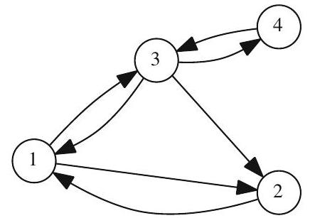
First try: let’s just count the number of backlinks, and make that the page’s rank.

Any potential downsides to this?

This can easily be gamed just by making many links to a page!

In the next try, we will taking into account the ranking of the pages who link to us.

Second try: rank pages by how many incoming links they have and how highly ranked they are.

For page i let x_{i} be its score and L_{i} be the set of all indices of pages linking to it. Then \begin{equation*} x_{i}=\sum_{x_{j} \in L_{i}} x_{j} \end{equation*}

Notice: you can’t just look at the graph anymore and know what the rankings will be! The ranking for one page depends on the rankings of all the others.

But it’s still easy to game this system, by setting up a set of interlinked pages and then making a ton of outgoing links to pages we want to promote.

Now we will downweight pages that have many many outgoing links.

Third try: downweight incoming links from pages that have many outgoing links.

For page j let n_{j} be its total number of outgoing links on that page. Then its score is

\begin{equation*} x_{i}=\sum_{x_{j} \in L_{i}} \frac{x_{j}}{n_{j}} \end{equation*}

:::

Working through PageRank: try 3

\begin{equation*} x_{i}=\sum_{x_{j} \in L_{i}} \frac{x_{j}}{n_{j}} \end{equation*}

Write down the system of equations this gives us. Then make it in an augmented matrix.

\begin{aligned} & x_{1}=\frac{x_{2}}{1}+\frac{x_{3}}{3} \\ & x_{2}=\frac{x_{1}}{2}+\frac{x_{3}}{3} \\ & x_{3}=\frac{x_{1}}{2}+\frac{x_{4}}{1} \\ & x_{4}=\frac{x_{3}}{3} . \end{aligned}

Augmented matrix:

import sympy as sym
P = sym.Matrix([[1,-1,-1,0,0],[-1,1,-1,0,0],[-1,0,1,-1,0],[0,0,-1,1,0]])
P

\displaystyle \left[\begin{matrix}1 & -1 & -1 & 0 & 0\\-1 & 1 & -1 & 0 & 0\\-1 & 0 & 1 & -1 & 0\\0 & 0 & -1 & 1 & 0\end{matrix}\right]

Set up the environment. Import the sympy library.

import sympy as sym

We make a matrix using the sym.Matrix function.

T = sym.Matrix([[1,2,3],[2,1,3],[2,1,1]])
T

\displaystyle \left[\begin{matrix}1 & 2 & 3\\2 & 1 & 3\\2 & 1 & 1\end{matrix}\right]

We can create symbolic variables, and put them into the matrix if we want…

x1=sym.var('x1'); x2=sym.var('x2');x3=sym.var('x3');x4=sym.var('x4')

x1

\displaystyle x_{1}

T2 = sym.Matrix([[1,x2,3],[2,1,3],[2,x1,1]])
T2

\displaystyle \left[\begin{matrix}1 & x_{2} & 3\\2 & 1 & 3\\2 & x_{1} & 1\end{matrix}\right]

If we input fractions, they are by default converted to floating point numbers:

T3 = sym.Matrix([[1,x2,1/3],[2,1,3],[2,x1,1]])
T3

\displaystyle \left[\begin{matrix}1 & x_{2} & 0.333333333333333\\2 & 1 & 3\\2 & x_{1} & 1\end{matrix}\right]

It’s nicer to input fractions and keep them as fractions:

T4 = sym.Matrix([[1,x2,sym.Rational(1,3)],[2,1,3],[2,x1,1]])
T4

\displaystyle \left[\begin{matrix}1 & x_{2} & \frac{1}{3}\\2 & 1 & 3\\2 & x_{1} & 1\end{matrix}\right]

We can substitute values in for variables:

T4.subs(x1,5)

\displaystyle \left[\begin{matrix}1 & x_{2} & \frac{1}{3}\\2 & 1 & 3\\2 & 5 & 1\end{matrix}\right]

We can find reduced row echelon form:

T4.rref()

(Matrix([
 [1, 0, 0],
 [0, 1, 0],
 [0, 0, 1]]),
 (0, 1, 2))

This outputs the RREF and tells us which columns correspond to bound variables.

Lastly, we can do Gauss-Jordan elimination to solve a system of equations with a matrix and a right-hand-side:

T4.gauss_jordan_solve(sym.Matrix([2,1,3]))

(Matrix([
 [(17*x1 - 24*x2 - 3)/(7*x1 - 12*x2 - 1)],
 [                 -4/(7*x1 - 12*x2 - 1)],
 [(-9*x1 + 12*x2 + 3)/(7*x1 - 12*x2 - 1)]]),
 Matrix(0, 1, []))

That’s messy! It’s exporting several things, but the one we want is the first.

T4.gauss_jordan_solve(sym.Matrix([2,1,3]))[0]

\displaystyle \left[\begin{matrix}\frac{17 x_{1} - 24 x_{2} - 3}{7 x_{1} - 12 x_{2} - 1}\\- \frac{4}{7 x_{1} - 12 x_{2} - 1}\\\frac{- 9 x_{1} + 12 x_{2} + 3}{7 x_{1} - 12 x_{2} - 1}\end{matrix}\right]

Now you try!

Create a matrix representing the system of equations for the “third try” in the PageRank problem:

\begin{aligned} & x_{1}=\frac{x_{2}}{1}+\frac{x_{3}}{3} \\ & x_{2}=\frac{x_{1}}{2}+\frac{x_{3}}{3} \\ & x_{3}=\frac{x_{1}}{2}+\frac{x_{4}}{1} \\ & x_{4}=\frac{x_{3}}{3} . \end{aligned}

# your code here

Now find the RREF form of this matrix. What does that tell you about the system?

# your code here

Next, use the gauss_jordan_solve. What’s surprising (or not) about these results?

# your code here

Substitute a specific value to get a particular solution…

JupyterLab

https://tinyurl.com/stat24320notebook1

Now what about the second try?

Remember this was our ‘second try’: \begin{equation*} x_{i}=\sum_{x_{j} \in L_{i}} x_{j} \end{equation*}

This was the system of equations. \begin{aligned} & x_{1}=x_{2}+x_{3} \\ & x_{2}=x_{1}+x_{3} \\ & x_{3}=x_{1}+x_{4} \\ & x_{4}=x_{3} . \end{aligned}

What happens if we try to solve this? Try it in Python.

What happens is that we get only the trivial solution, where all the ranks are zero. This makes sense because it is a homogeneous system with full rank.

Diffusion

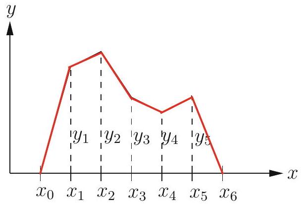
Discretizing continuous functions

• Rod with fixed temperatures y_{left} and y_{right} at each end, internal heat source given as f(x), 0 \leq x \leq 1

• What’s the temperature at each point along the length?

Discrete approximation to temperature function (n=5)

• equally spaced points, called nodes, x_{0}=0, x_{1}, x_{2}, \ldots, x_{n+1}=1, distance h apart.
• heat on the i th segment \approx temperature at its left node.
• temperature is y(x), y_{i}=y\left(x_{i}\right).

Equations to balance the flow of heat from each node to its neighbors:

\begin{equation*} -y_{i-1}+2 y_{i}-y_{i+1}=\frac{h^{2}}{K} f\left(x_{i}\right) \end{equation*}

Suppose:

• rod of material with K=1 on x-axis, for 0 \leq x \leq 1.
• known internal heat source f(x)
• left and right ends of the rod are held at 0{ }^{\circ} \mathrm{C} (degrees Celsius)
• n=5 nodes

What are the discretized steady-state equations?

• x_{i}=i h.
• y_{0} is given to be 0, dissapears
• y_{n+1}=y_{6} =0,Thus we have from equation (1.2) five equations in the unknowns y_{i}, i=1,2, \ldots, 5

\begin{array}{lllllr} 2 y_{1}&-y_{2} & & & & =f(1 / 6) / 36 \\ -y_{1}&+2 y_{2}&-y_{3} & & & =f(2 / 6) / 36 \\ &-y_{2}&+2 y_{3}&-y_{4} & & =f(3 / 6) / 36 \\ &&-y_{3}&+2 y_{4}&-y_{5} & =f(4 / 6) / 36 \\ &&&-y_{4}&+2 y_{5} & =f(5 / 6) / 36 \end{array}

This is already a pain to work with by hand!

Build the matrix representing the system of equations:

N=6
M = sym.zeros(N)
for i in range(N):
  if (i>0):
      M[i-1,i]=-1
  M[i,i]=2
  if (i<N-1):
      M[i+1,i]=-1
M

\displaystyle \left[\begin{matrix}2 & -1 & 0 & 0 & 0 & 0\\-1 & 2 & -1 & 0 & 0 & 0\\0 & -1 & 2 & -1 & 0 & 0\\0 & 0 & -1 & 2 & -1 & 0\\0 & 0 & 0 & -1 & 2 & -1\\0 & 0 & 0 & 0 & -1 & 2\end{matrix}\right]

\begin{equation*} -y_{i-1}+2 y_{i}-y_{i+1}=\frac{h^{2}}{K} f\left(x_{i}\right) \end{equation*}

Decide on a function for f. Let’s say \frac{h^{2}}{K} f = x_i^2.

Say that x is running from 0 to 1. Then we can have

import numpy as np
x=np.arange(0,1,1/N)
f=x**2
x=sym.Matrix(x)
f=sym.Matrix(f)

sol=M.gauss_jordan_solve(f)
sol[0]

\displaystyle \left[\begin{matrix}0.416666666666667\\0.833333333333333\\1.22222222222222\\1.5\\1.52777777777778\\1.11111111111111\end{matrix}\right]

Now you

1. Implement this yourself in Python
2. Make a plot of the output (you’ll want to use PyPlot)
3. Increase N and make more plots
4. This was assuming the temperature at the ends was 0. How can we change this?

Reaction-Diffusion in Biology

Turing pattern formation

https://colab.research.google.com/github/ijmbarr/turing-patterns/blob/master/turing-patterns.ipynb#scrollTo=GsEPBsz33E14