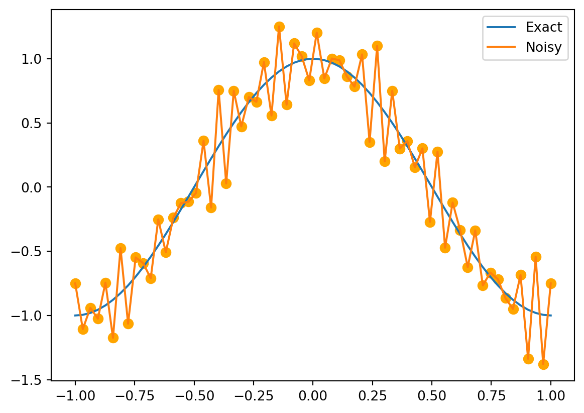
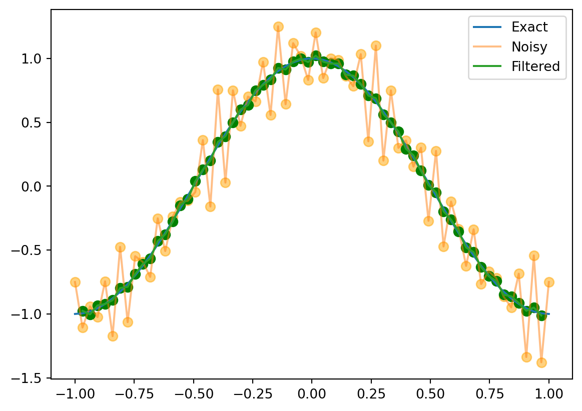
y = np.zeros_like(x)for k inrange(1, 63): y[k] =1/4*g(x[k+1]) +1/2*g(x[k]) +1/4*g(x[k-1])plt.plot(x, f(x), label='Exact')plt.plot(x, g(x), label='Noisy', alpha=0.5)plt.scatter(x, g(x), color='orange', s=50, alpha=0.5) # Add dots for 'Noisy'plt.plot(x[1:-1], y[1:-1], label='Filtered')plt.scatter(x[1:-1], y[1:-1], color='green', s=50) # Add dots for 'Filtered'plt.legend()
. . .
This captured the low-frequency part of the signal, and filtered out the high-frequency noise. That’s just what we wanted! This is called a low-pass filter.
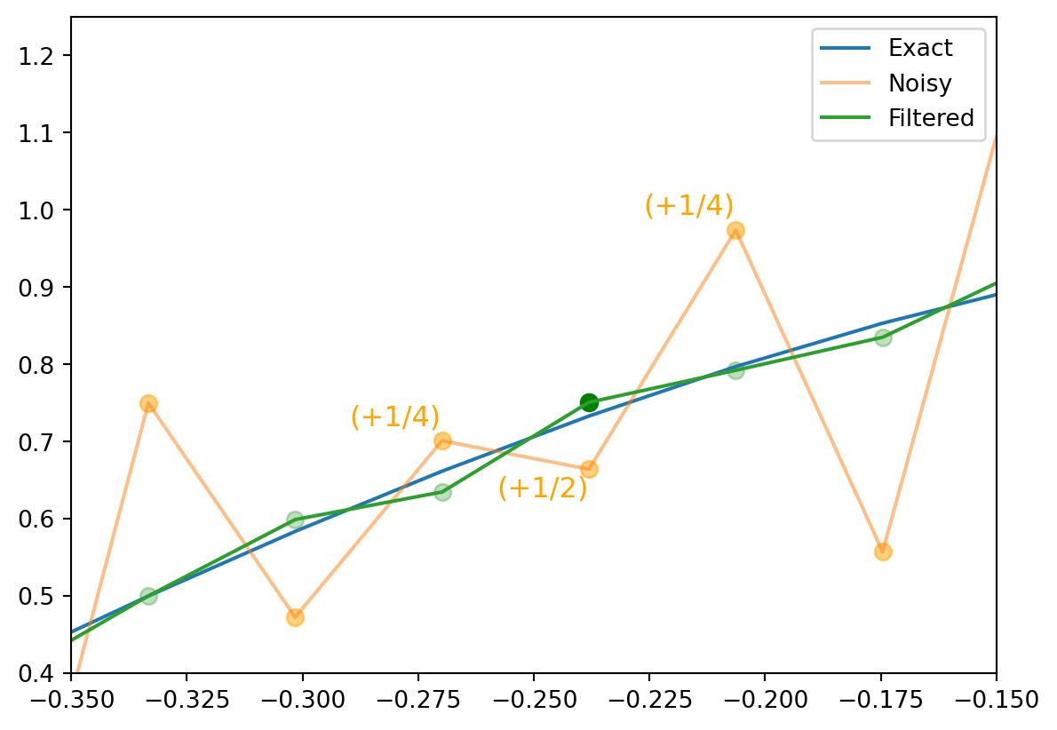
We can zoom in on a few points to see the effect of the filter.
plt.plot(x, f(x), label='Exact')plt.plot(x, g(x), label='Noisy', alpha=0.5)plt.scatter(x, g(x), color='orange', s=50, alpha=0.5) # Add dots for 'Noisy'plt.plot(x, y, label='Filtered')for i inrange(len(x)):if i ==24: plt.scatter(x[i], y[i], color='green', s=50, alpha=1) # Add dot for y[24] with 100% opacityelse: plt.scatter(x[i], y[i], color='green', s=50, alpha=0.25) # Add other dots for 'Filtered' with 25% opacityplt.text(x[25]-.02, g(x[25])+.02, '(+1/4)', color='orange', fontsize=12) # Add label to the orange dot at 24plt.text(x[24]-.02, g(x[24])-.035, '(+1/2)', color='orange', fontsize=12) # Add label to the orange dot at 24plt.text(x[23]-.02, g(x[23])+.02, '(+1/4)', color='orange', fontsize=12) # Add label to the orange dot at 24plt.xlim(-0.35, -.15)# make the ylim automatically adjust to the data in the zoomed in regionplt.ylim(bottom=0.4, top=1.25)plt.legend()
Now you try
See if you can make a figure which will just find the noisyness…
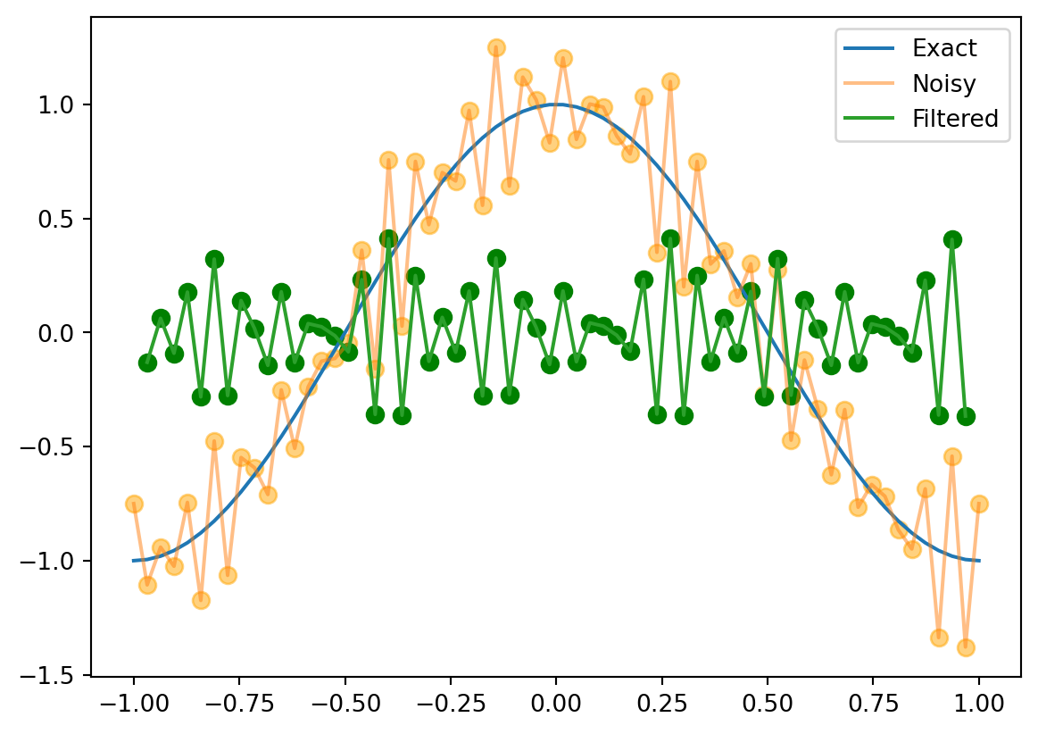
A different filter
What if we subtract the values at \(x_{k+1}\) and \(x_{k-1}\) instead of adding them?
y = np.zeros_like(x)for k inrange(1, 63): y[k] =-1/4*g(x[k+1]) +1/2*g(x[k]) -1/4*g(x[k-1])plt.plot(x, f(x), label='Exact')plt.plot(x, g(x), label='Noisy', alpha=0.5)plt.scatter(x, g(x), color='orange', s=50, alpha=0.5) # Add dots for 'Noisy'plt.plot(x[1:-1], y[1:-1], label='Filtered')plt.scatter(x[1:-1], y[1:-1], color='green', s=50) # Add dots for 'Filtered'plt.legend()
. . .
This is a high-pass filter. It captures the high-frequency noise, but filters out the low-frequency signal.
Inverse Matrices
Definition of inverse matrix
Let \(A\) be a square matrix.
Inverse for \(A\) is a square matrix \(B\) of the same size as \(A\)
such that \(A B=I=B A\).
If such a \(B\) exists, then the matrix \(A\) is said to be invertible.
Also called “singular” (non-invertible), or “nonsingular” (invertible)
Conditions for invertibility
Conditions for Invertibility The following are equivalent conditions on the square \(n \times n\) matrix \(A\) :
The matrix \(A\) is invertible.
There is a square matrix \(B\) such that \(B A=I\).
The linear system \(A \mathbf{x}=\mathbf{b}\) has a unique solution for every right-hand-side vector \(\mathbf{b}\).
The linear system \(A \mathbf{x}=\mathbf{b}\) has a unique solution for some right-hand-side vector \(\mathbf{b}\).
The linear system \(A \mathbf{x}=0\) has only the trivial solution.
\(\operatorname{rank} A=n\).
The reduced row echelon form of \(A\) is \(I_{n}\).
The matrix \(A\) is a product of elementary matrices.
There is a square matrix \(B\) such that \(A B=I\).
Elementary matrices
Each of the operations in row reduction can be represented by a matrix \(E\).
. . .
Remember: - \(E_{i j}\) : The elementary operation of switching the ith and jth rows of the matrix. - \(E_{i}(c)\) : The elementary operation of multiplying the ith row by the nonzero constant \(c\). - \(E_{i j}(d)\) : The elementary operation of adding \(d\) times the jth row to the ith row.
. . .
Find an elementary matrix of size \(n\) is by performing the corresponding elementary row operation on the identity matrix \(I_{n}\).
. . .
Example: Find the elementary matrix for \(E_{13}(-4)\)
. . .
Add -4 times the 3rd row of \(I_{3}\) to its first row…
If we perform the elementary operation \(E\) on the superaugmented matrix, we get the matrix \(E\) in the augmented part:
. . .
\[
E[A \mid I]=[E A \mid E I]=[E A \mid E]
\]
. . .
This can help us keep track of our operations as we do row reduction
The augmented part is just the product of the elementary matrices that we have used so far.
Now continue applying elementary row operations until the part of the matrix originally occupied by \(A\) is reduced to the reduced row echelon form of \(A\).
\(B=E_{k} E_{k-1} \cdots E_{1}\) is the product of the various elementary matrices we used.
Inverse Algorithm
Given an \(n \times n\) matrix \(A\), to compute \(A^{-1}\) :
Form the superaugmented matrix \(\widetilde{A}=\left[A \mid I_{n}\right]\).
Reduce the first \(n\) columns of \(\tilde{A}\) to reduced row echelon form by performing elementary operations on the matrix \(\widetilde{A}\) resulting in the matrix \([R \mid B]\).
If \(R=I_{n}\) then set \(A^{-1}=B\); otherwise, \(A\) is singular and \(A^{-1}\) does not exist.
2x2 matrices
Suppose we have the 2x2 matrix
\[
A=\left[\begin{array}{ll}
a & b \\
c & d
\end{array}\right]
\]
. . .
Do row reduction on the superaugmented matrix:
\[
\left[\begin{array}{ll|ll}
a & b & 1 & 0 \\
c & d & 0 & 1
\end{array}\right]
\]
. . .
\[
A^{-1}=\frac{1}{D}\left[\begin{array}{rr}
d & -b \\
-c & a
\end{array}\right]
\]
for page \(j\) let \(n_{j}\) be its total number of outgoing links on that page.
Then the score for vertex \(i\) is the sum of the scores of all vertices \(j\) that link to \(i\), divided by the total number of outgoing links on page \(j\). . . . \[
x_{i}=\sum_{x_{j} \in L_{i}} \frac{x_{j}}{n_{j}}
\]
We can introduce a correction vector, equivalent to adding links from the dangling node to every other node, or to all connecting nodes (via some path).